Prediction of Commuter Vehicle Demand Torque Based on Historical Speed Information

Shiji Sun, Mingxin Kang, Yuzhe Li

Abstract: The development of vehicle-to-everything and cloud computing has brought new opportunities and challenges to the automobile industry. In this paper, a commuter vehicle demand torque prediction method based on historical vehicle speed information is proposed, which uses machine learning to predict and analyze vehicle demand torque. Firstly, the big data of vehicle driving is collected, and the driving data is cleaned and features extracted based on road information. Then, the vehicle longitudinal driving dynamics model is established. Next, the vehicle simulation simulator is established based on the longitudinal driving dynamics model of the vehicle, and the driving torque of the vehicle is obtained. Finally, the travel is divided into several accelerationcruise-deceleration road pairs for analysis, and the vehicle demand torque is predicted by BP neural network and Gaussian process regression.

Keywords: demand torque prediction; commuter vehicle; historical driving data; machine learning

1 Introduction

In recent years, the development of information and communication technologies such as big data, cloud computing, vehicle-to-everything, and intelligent transportation system has brought new opportunities and challenges to the automobile industry [1]. Traditional automobile manufacturers are also adapting to the requirements of new technology development and carrying out research on optimal scheduling and real-time optimal control of intelligent networked vehicles in the era of data interconnection. However, the automobile engine is a complex multivariable coupling system with complex characteristics such as nonlinearity, intricate modeling, time delay, random uncertainty, and so on. Therefore,it is challenging to create an accurate model based purely on physical or mathematical principles [2] .

Some computational simulation approaches are adopted to model the engine operation [3, 4],and the torque of the engine is obtained by simulation. In [5], the nonlinear model of the vehicle is linearized, and a linear time-varying algorithm is adopted to solve the problem. However, the vehicle demand torque is not predicted, and the vehicle speed is directly input into the prediction model. In [6], Sun uses the exponential forecasting method to forecast the demand torque.Although the calculation is simple, the forecasting accuracy is low. In [7], Jiang uses the autoregressive model to predict the driver’s demand torque and predicts the driver's demand torque in the next period according to the driver’s demand torque in the previous period. In [8], a road network topology model is established to predict short-term traffic flow, but other vehicle driving characteristics are not analyzed and predicted.

The rapid development of machine learning has brought new data regression prediction analysis methods, such as BP neural network [9] and Gaussian process regression [10]. The artificial neural networks model can acquire the essence of data by adaptive adjusting model parameters in self-learning to achieve a better prediction effect[11] . In [12], BP neural network is used to analyze and predict the required torque of vehicles.Typically, the more historical data is used, the more accurate the prediction is. In [13], Park uses machine learning of optimal control parameters for predictive control of vehicles. In [14], a long short-term memory neural network method is used to predict traffic speed.

The driving torque of commuter vehicles is of great significance for improving ride comfort,energy saving, and emission reduction. In this paper, based on the historical driving big data of commuter vehicles, the demand torque of vehicle is predicted and analyzed. Furthermore, a new storage and analysis method for vehicle driving big data is proposed. As shown in Fig. 1, commuter vehicle upload driving data information to the cloud server, where driving data can be statistically analyzed, simulated, and predicted.Then the expected demand torque can be sent to commuter vehicle.

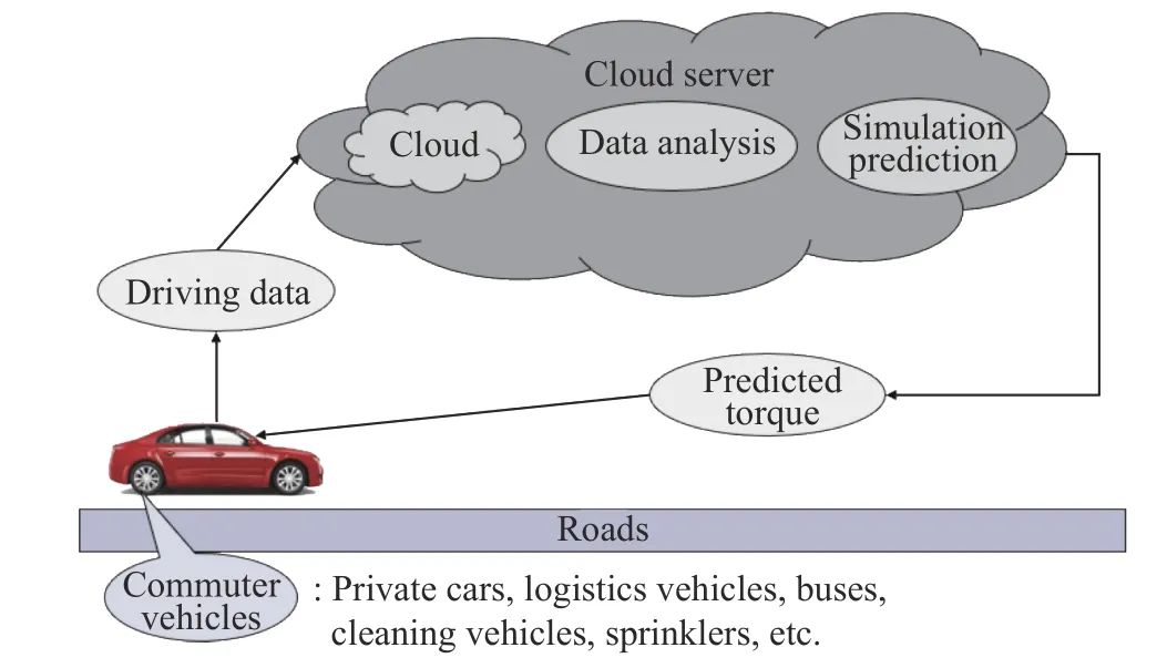
Fig. 1 Data storage and analysis method

The work done in this paper is summarized as follows: Firstly, the speed information of commuter vehicles for 20 days is collected, and the interpolation function is used to convert the time-based sampling data into the distance-based sampling data. Then, data cleaning and feature extraction are carried out to eliminate invalid sampling data, and the effective driving information of the vehicle for 14 days is obtained. Next,the vehicle driving dynamics model is established, and the vehicle simulator is built in MATLAB based on the selected model. By inputting the vehicle driving data into the vehicle simulator, the driving torque of the vehicle can be obtained. Finally, the travel is divided into several acceleration-cruise-deceleration sections to analyze the torque, using BP neural network and Gaussian process regression method to predict the vehicle demand torque.

2 Analysis and Preprocessing of Vehicle Driving Data

2.1 Vehicle Driving Data Acquisition

The research objective of this paper is the commuter vehicle with fixed driving routes, such as sprinklers, cleaning vehicles, logistics vehicles,etc. Commuter vehicles have a fixed driving route, which is very common in our daily life.Therefore, it is significant to study the driving characteristics of the commuter vehicle. It is necessary to collect and analyze the driving data of vehicles with fixed driving routes.

This paper chooses the suburban section of Tokyo, Japan, for data collection and carries out the cycle driving measurement of the running passenger car, and the measurement days are 20 days. The vehicle travels in one direction from home to the office every day, with about 14.6km.The commuter route is shown in Fig. 2, and the blue route in Fig. 2 is our measured driving route.

We borrow Global Positioning System(GPS) and Controller Area Network (CAN) for data acquisition. Driving data is measured by GPS and CAN and uploaded to the cloud server.Because the volume of data is large and the realtime requirement of data transmission is high,the data collection only includes the speed and location information of commuter vehicles. The sampling frequency is 0.02 s, and the total sample is 20 days. In addition, the collected data include the altitude of the road and the slope information of the road surface, as shown in Fig. 3.

Fig. 2 The route track of commuting

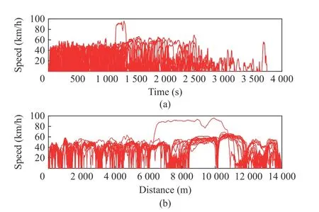
Fig. 4 Vehicle sampling data images: (a) time sampling; (b)distance sampling

Fig. 3 Road altitude and slope change maps: (a) altitude; (b)slope

2.2 Data Analysis and Preprocessing

Firstly, the 20-day driving data is visualized.Then, the original data is sampled based on time,and the sampling time is 0.02 s. Next, the data is converted to speed sampling based on the distance to better observe the commuter vehicle driving characteristics. Finally, the interpolation function is used to interpolate the distance, and the sampling interval is 1 m. The raw data based on time sampling and the data based on distance sampling are shown in Fig. 4.

The original data based on time sampling is messy, and the characteristics of the data can’t be seen. On the other hand, the data based on distance sampling can see certain regularity,which is convenient for analyzing the driving characteristics of vehicles.

There may be data loss or anomaly in the actual data sampling process, and the data with problems is defined as invalid data. As shown in Fig. 5, the 20-day driving big data is divided into our groups for analysis. For example, the distance from home to office is about 14 000 m.Still, the sampling distance of some invalid data s only about 3 500 m, so it is necessary to eliminate these unsatisfied invalid data.

After data analysis and preprocessing, there are 14 days of valid data in the 20-day driving big data. As shown in Fig. 6, the 14-day valid data is based on the distance sampling distance speed image. Through the distance speed image,we can intuitively see the driving characteristics of commuter cars in the driving process, and the overall driving image presents certain regularity.

The commuter car starts during the driving process, and the speed increases from zero to the required value, and then keeps a certain speed to continue driving. However, commuter cars will slow down or brake to stop when encountering traffic lights or special road conditions. This driving characteristic of the commuter car can be expressed by the acceleration-cruise-deceleration process.

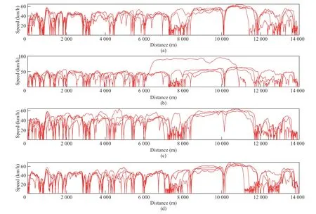
Fig. 5 Sampled data analysis images: (a) 1-5; (b) 6-10; (c) 11-15; (d) 16-20

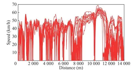
Fig. 6 Effective sampled data image

3 Torque Analysis Based on Vehicle Dynamics Model

3.1 Longitudinal Dynamics Model of Vehicle

Vehicle driving dynamics calculates the power consumed when the vehicle passes through a specific route by estimating aerodynamic resistance,rolling resistance, climbing resistance, and driver behavior. The driving data of commuter cars are obtained by sampling, and the big data of car driving contains the speed information. However,this information to analyze the driving characteristics of the whole vehicle is far from enough, so it is necessary to study the driving dynamics modeling of the car through the Simulink module of MATLAB software to simulate our commuter car. In this paper, the longitudinal driving dynamics model of the vehicle proposed by [15] is adopted when analyzing the vehicle's driving dynamics, as shown in Fig. 7.

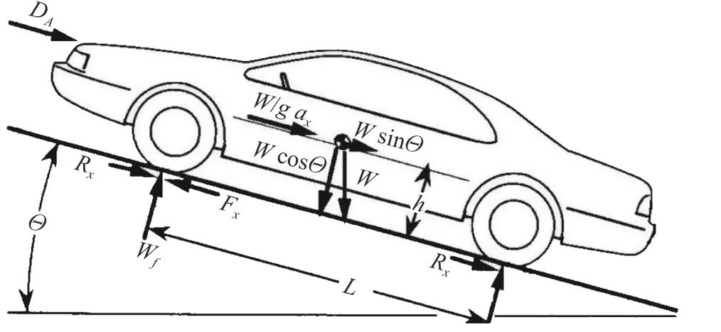
Fig. 7 Force analysis of vehicle from [15]

The longitudinal motion of the vehicle can be described by the travelling distances, the velocityvand the longitudinal accelerationax:

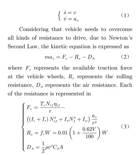
and the meanings of symbols are shown in Tab. 1.

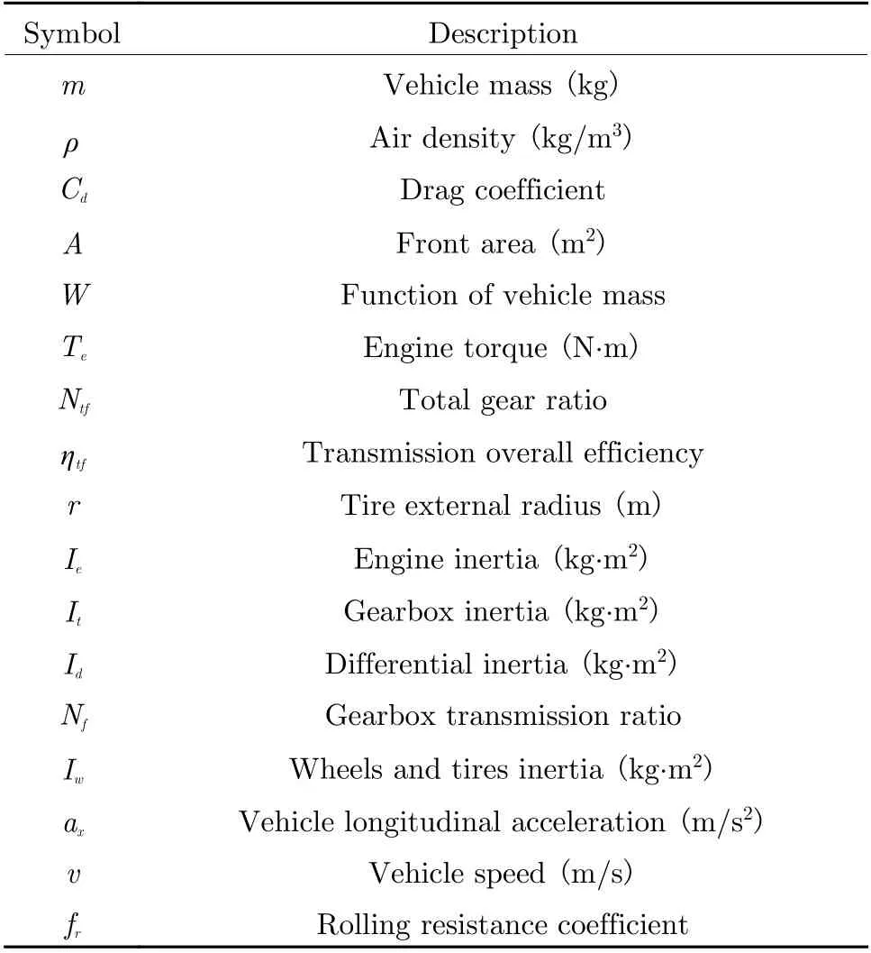
Tab. 1 Vehicle parameters

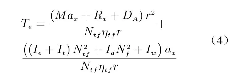
In addition, the engine torque can be expressed by

3.2 Torque Model Based on Dynamic

After getting the vehicle driving dynamics model,the model needs to be simulated, and the Simulink module in MATLAB software is selected to build the commuter vehicle model.Then, combined with the dynamic model analysis of the previous module, the program is written in MATLAB to build the model. Finally, the built driver-engine-vehicle-route control loop simulation program is used to simulate the automobile motion model, as shown in Fig. 8.

All driving modules of the vehicle, such as the driving module, engine module, vehicle driving dynamics module, etc., are built into the vehicle simulation simulator, as shown in Fig. 9.

Through the simulation simulator, the 14-day required torque of the vehicle can be obtained after inputting the big data of 14-day vehicle driving.

4 Prediction and Analysis of Vehicle Demand Torque

4.1 Demand Torque Analysis

Commuter vehicles will encounter red street lights, road congestion, pedestrians passing through intersections, etc. Therefore, many starting, cruising, and stopping processes will be driving. Multiple acceleration-cruise-deceleration sections can represent the driving process of commuter vehicles, so a typical section can be selected to analyze the driving characteristics of vehicles.

In this paper, a typical road section from 10 km to 11.5 km is selected to forecast and analyze the vehicle demand torque. The vehicle driving torque has been obtained through the vehicle simulation simulator. Next, BP neural network and Gaussian process regression are used to predict the vehicle demand torque.

4.2 Back Propagation Neural Network Prediction

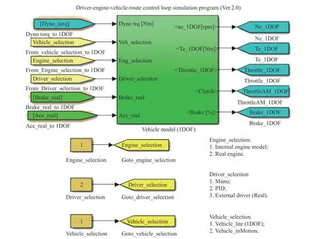
Fig. 8 Vehicle simulation simulator

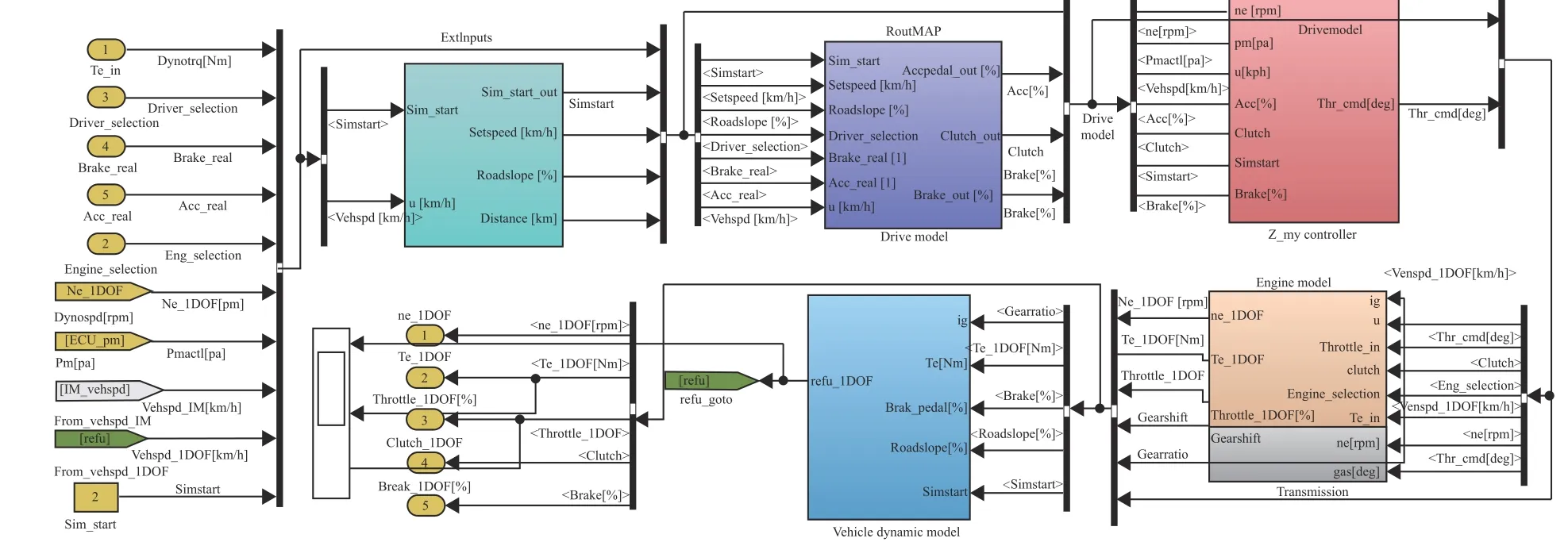
Fig. 9 Driving modules of vehicle

Back propagation neural network, also known as the error backpropagation algorithm, is the most successful neural network learning algorithm.Through the training of sample data, the network weights and thresholds are constantly modified to make the error function descend along the negative gradient direction and approach the expected output. It is a widely used neural network model used primarily in function approximation, model recognition and classification, data compression, and time series prediction.

According to algorithm 1, BP neural network is built to predict and analyze the demand torque. Among them, the training time is set to 1 000 times, and the learning rate is set to 0.01.

Algorithm 1: Back propagation neural network Input: Training set D , learning rate α 1: Function BP(D, α)

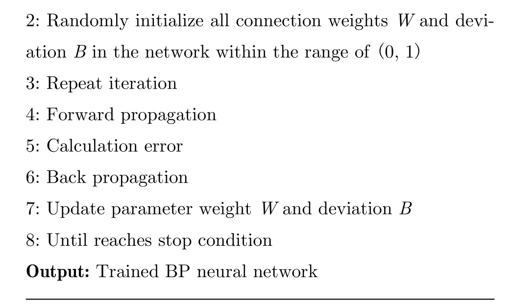
2: Randomly initialize all connection weights W and deviation B in the network within the range of (0, 1)3: Repeat iteration 4: Forward propagation 5: Calculation error 6: Back propagation 7: Update parameter weight W and deviation B 8: Until reaches stop condition Output: Trained BP neural network

The prediction results of the BP neural network are shown in Fig. 10. The solid red line is the actual torque of the vehicle, and the dashed blue line is the predicted demand torque.

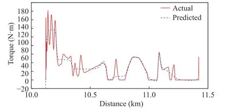
Fig. 10 Demand torque predicted by BP neural network

The correlation coefficient in the training process is shown in Fig. 11, and the correlation coefficient of predicted demand torque is 0.885 89.

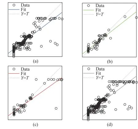
Fig. 11 Regression analysis diagrams of predicted torque: (a)training: R=0.873 4; (b) validation R=0.939 23; (c)test: R=0.902 84; (d) all: R=0.885 89

It can be seen that although the BP neural network has high nonlinearity and strong generalization ability, it also has some shortcomings,such as slow convergence speed, many iterative steps, easy falling into a local minimum, and poor global search capability.

4.3 Gaussian Process Regression Prediction

Gaussian process is a new machine learning algorithm based on statistical learning theory and Bayesian theory, often used to solve regression and classification problems.

Gaussian process regression can be expressed as

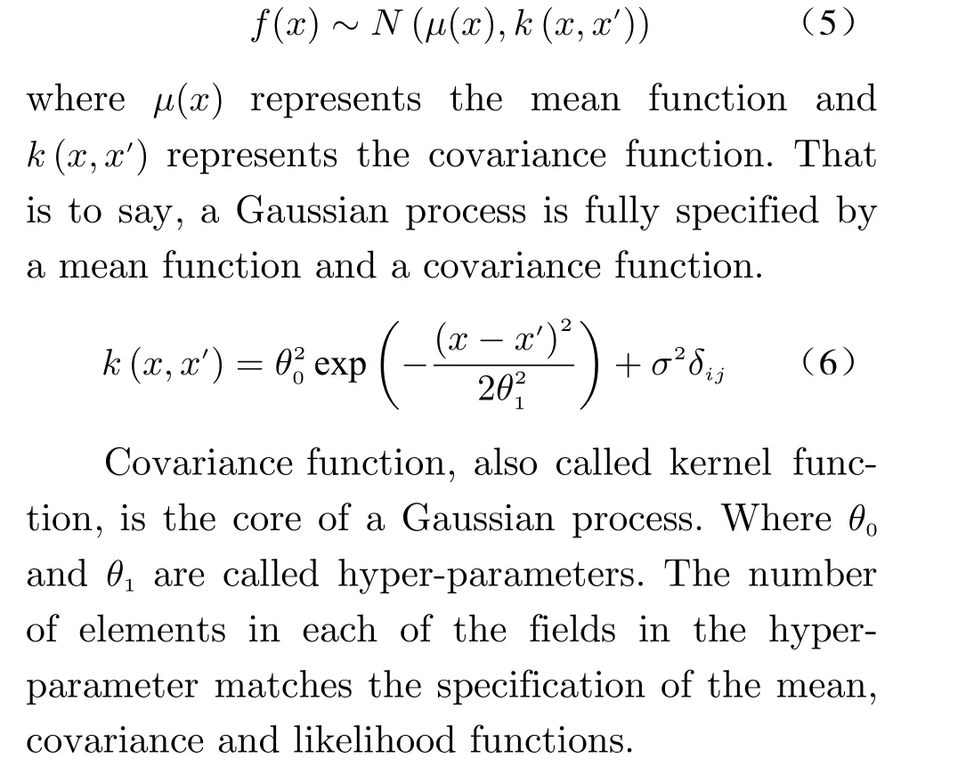
Gaussian process regression can be understood as finding any set of functions from countless functions that conform to the test data set.According to the prior information of a set of data sets, the range of the function set is continuously narrowed. The distribution of the function set is calculated by Bayesian method and Gaussian distribution property. According to the distribution of the obtained function set, the subsequent data are predicted.

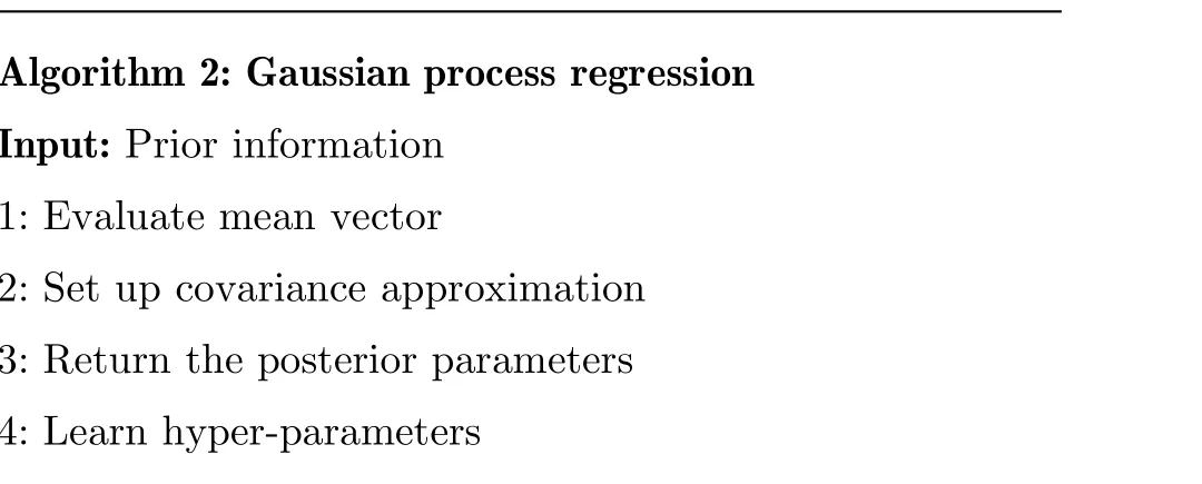
Algorithm 2: Gaussian process regression Input: Prior information 1: Evaluate mean vector 2: Set up covariance approximation 3: Return the posterior parameters 4: Learn hyper-parameters

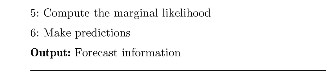
5: Compute the marginal likelihood 6: Make predictions Output: Forecast information

According to algorithm 2, Gaussian process regression is used to regress and predict the vehicle demand torque, and the prediction result is shown in Fig. 12. The solid red line is the real torque of the vehicle, and the dashed blue line is the predicted demand torque. It can be seen that the prediction of demand torque by Gaussian process regression is more accurate.

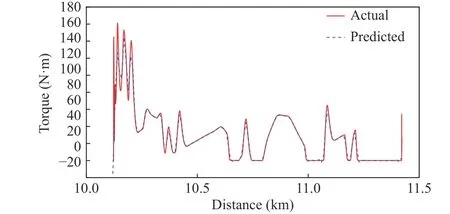
Fig. 12 Demand torque predicted by Gaussian process

5 Conclusion

Based on the historical speed information of commuter vehicles, the demand torque of commuter vehicles is predicted and analyzed in this paper.Firstly, the speed information of 20 days was collected, and the data were cleaned and feature extracted, and the effective driving data of 14 days was obtained. Then, a vehicle simulator is established based on vehicle driving dynamics,and the driving torque of the vehicle is obtained by simulation. Finally, the vehicle demand torque is predicted by BP neural network and Gaussian process regression.