Similarity solutions of Prandtl mixing length modelled two dimensional turbulent boundary layer equations

Bo-Hua Sun

School of Civil Engineering & Institute of Mechanics and Technology, Xi’an University of Architecture and Technology, Xi’an 710055, China

Keywords:Turbulent boundary layers Laminar boundary layers Similarity transformation Similarity solution Prandtl mixing length Reynolds number

ABSTRACT The exact similarity solutions of two dimensional laminar boundary layer were obtained by Blasius in 1908, however, for two dimensional turbulent boundary layers, no Blasius type similarity solutions (special exact solutions) have ever been found. In the light of Blasius’ pioneer works, we extend Blasius similarity transformation to the two dimensional turbulent boundary layers, and for a special case of flow modelled by Prandtl mixing-length, we successfully transform the two dimensional turbulent boundary layers partial differential equations into a single ordinary differential equation. The ordinary differential equation is numerically solved and some useful quantities are produced. For numerical calculations, a complete Maple code is provided.

The theory of laminar boundary layer (as shown in Fig. 1 ) dates back to almost 120 years ago [1,2] . In 1921, Prandtl discovered that almost all boundary-layer movements in nature are not only in laminar but also mainly in turbulence [3–8] . However, the understanding of fully developed turbulence remains a major unsolved problem in classic physics [9–21] .

For the laminar boundary layers, Blasius introduced a similarity transformation and found its solution [2] . The corresponding turbulent problem, i.e., the 2D turbulent boundary layers have been studied intensively by numerical integrations [3,4] .

For the free shear turbulent flows, Launder [20] and Townsend[21] proposed their similarity solutions. Since those free flows have no fixed walls, it means that the free shear turbulent flows are not belong to the turbulent boundary layers flows. Dixit and Ramesh[22] studied the pressure-gradient-dependent logarithmic laws in sink flow turbulent boundary layers by using perturbation method.

To the best of the author’s knowledge, no Blasius type similarity solutions of Prandtl mixing-length-modelled two-dimensional turbulent boundary layer equation have even been obtained. The question is whether the Blasius similarity transformation that used to solve the 2D laminar boundary layers could still be extended to the 2D turbulent boundary layers. If it were possible, how to formulate and what conditions must be hold. Those questions remain open.

In the light of Blasius’s pioneer work, we extend Blasius similarity transformation to the two dimensional turbulent boundary layers, successfully transform the two dimensional turbulent boundary layers’s partial differential equations into a single ordinary differential equation. To solve and numerically solve the ordinary differential equation, a complete Maple code is provided.

A thin flat plate is immersed at zero incidence in a uniform stream as shown in Fig. 1 , which flows with speedU(x)and is assumed not to be affected by the presence of the plate, except in the boundary layer. The fluid is supposed unlimited in extent,and the origin of coordinates is taken at the leading edge, withxmeasured downstream along the plate andyperpendicular to it.Assuming that the turbulent flow is steady with pressure gradient along thexaxis.

The Reynolds-averaged Navier–Stokes equations [5] of the two dimensional turbulent boundary layers flow under gradient,d¯p/dx,are reduced to

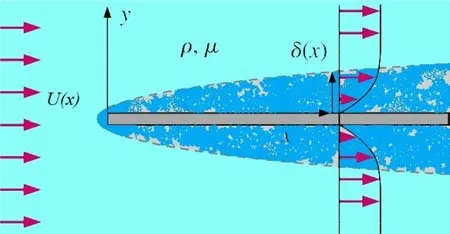
Fig. 1. Turbulent boundary layer.

and boundary conditions:

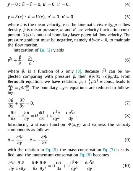
According to Blasius laminar boundary similarity theory [2,4] ,the system has no characteristic length, we can assume that the velocity profiles at different distances from the leading edge are affine or similarity to one another, i.e. that the velocity profile ¯uat different distancesxcan be mapped onto each other by suitable choice of scaling factors for ¯uandy. A suitable scaling factor for¯ucould be the free stream velocityU(x), while fory, “boundarylayer thickness”δ(x), which increases with distancex, could be used. The similarity law of the velocity profile can thus be written asu/ [δ(x)U] =f(η)withη=y/δ(x), where the functionf(η)is independent ofx.

Introducing following transformations

thus the velocity components become

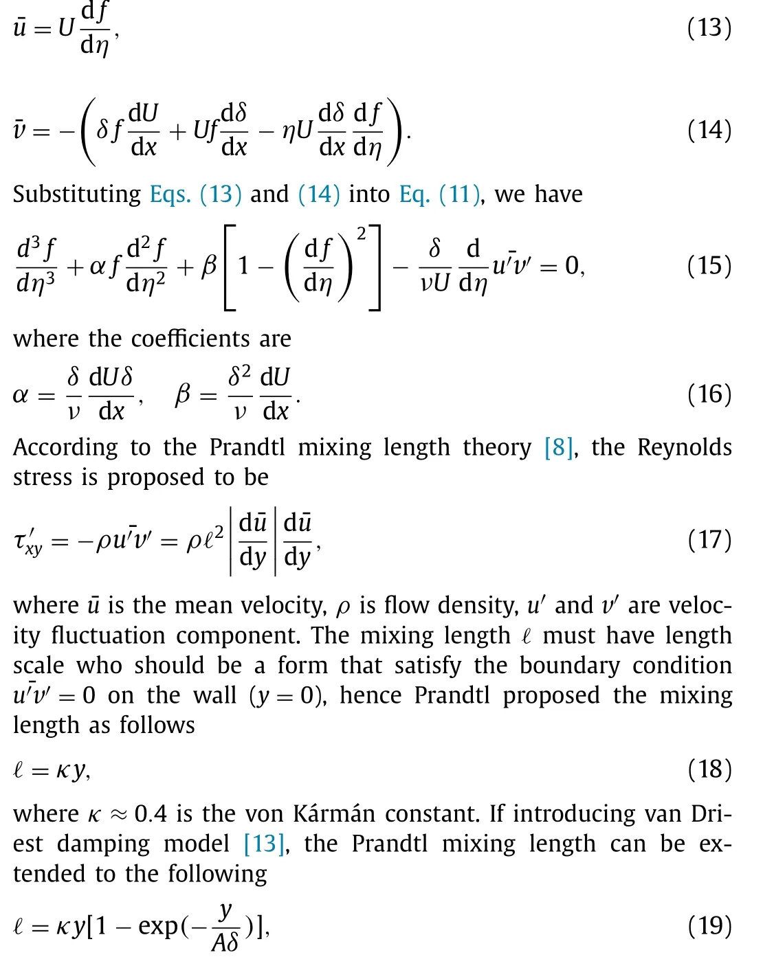
In this paper, all forthcoming formulations and numerical calculations are based on model in Eq. (18) instead of Eq. (19) , hence we have

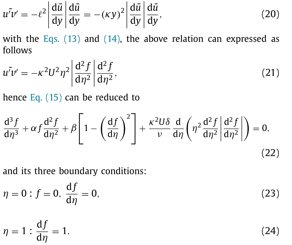
General speaking, the coefficients in Eq. (22) are the functions ofx, then there is no way to find similarity solutions in Eq. (22) .However, in the 3rd term of Eq. (22) , if we setUδas a constant,ie.,Uδ=C, leads to an interesting result, i.e.,α= 0 , and if the coefficientβis assumed to be constant

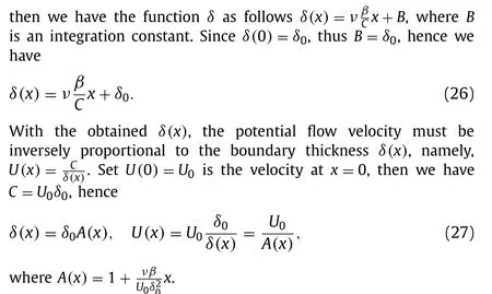
According to Schlichting [4] ,U(x)=U0 /A(x), which is the outside the boundary layer for convergent (β ＜0 ) or divergent (β ＞0 )radial motion between intersecting planes, respectively. The negative and positive sign indicates that the motion is towards to and away from the line of intersection. The laminar boundary layer motion due to convergent flow was discussed by Pohlhausen [23] .

Finally, we have successfully transformed the partial differential equations in Eq. (10) and its boundary conditions into a single ordinary differential equation as follows

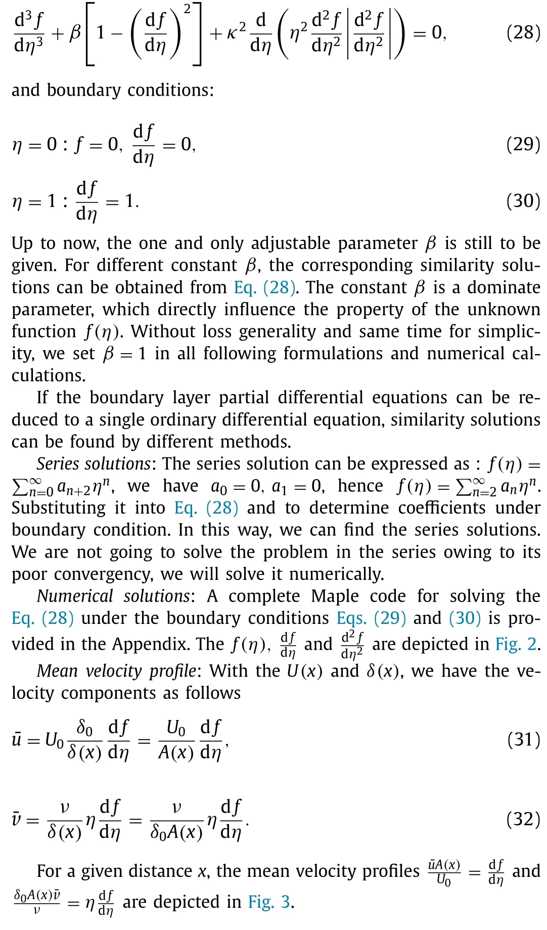
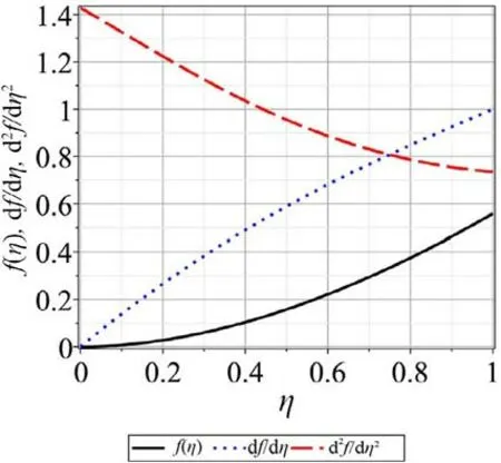
Fig. 2. f(η) ,and , in which f ′′ (0) = | η=0 = 1 . 4278 .

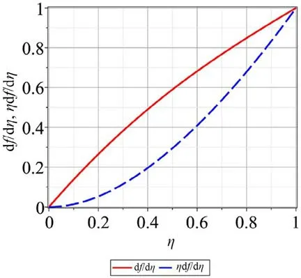
Fig. 3. Mean velocity profile in the case β = 1 . The red solid line is = , and blue dashline is = . (For interpretation of the references to colour in this figure legend, the reader is referred to the web version of this article.)

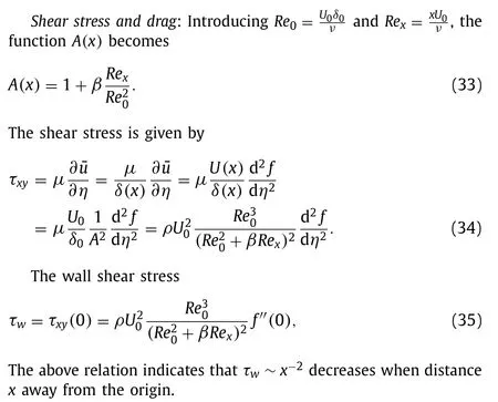
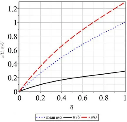
Fig. 4. Flow velocity ratios, in which the blue dot-line is ¯u /U, black solid line is u ′ /U and red long dashline is u/U. (For interpretation of the references to colour in this figure legend, the reader is referred to the web version of this article.)

The drag on one side of a plate of lengthLand unit breadth is then

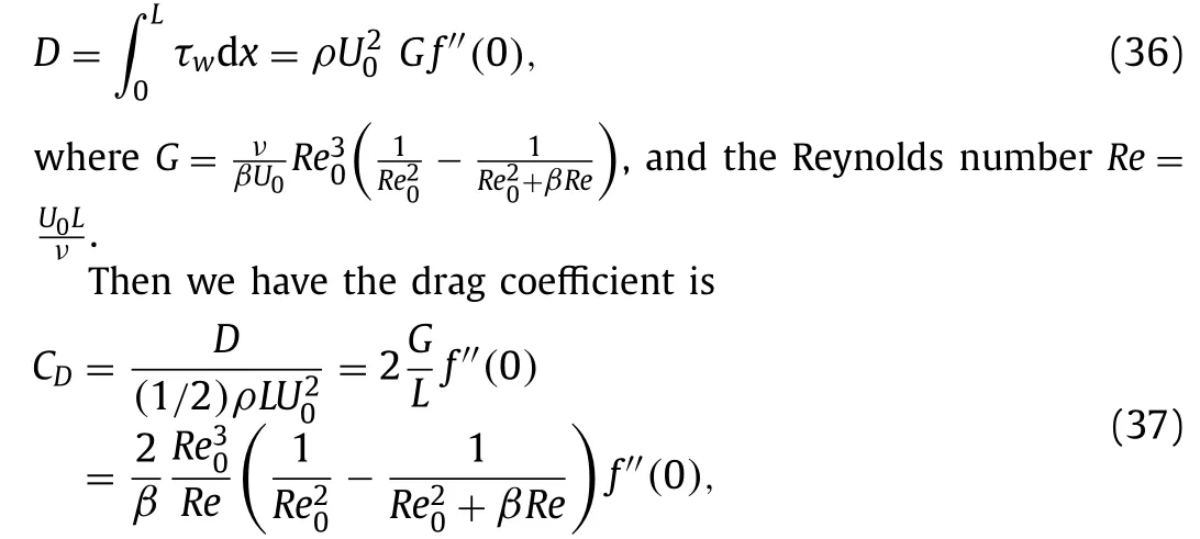
The above relation reveals that the drag coefficient is not only dependent on the Reynolds numberRebut alsoRe0 , owing to convergent/divergent nature of the flow.

Velocityfluctuationsandtotalvelocityfield: In Prandtl mixinglength theory [4,8] , Prandtl assumes a greatly simplified model of the fluctuations, according to which the individual fluid elements are displaced in a mean distance (the mixing length)ℓby the fluctuations, perpendicular to the main flow direction, but still retaining their momentum. The element that was initially aty, and is now aty+ℓ, has a higher velocity than its new surroundings. The velocity difference is a measure of the fluctuation velocity in thexdirection:

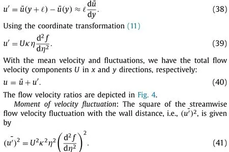
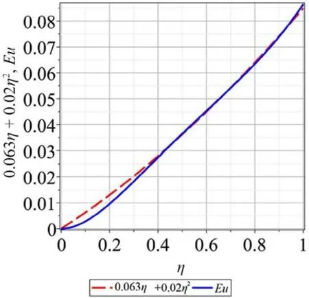
Fig. 5.

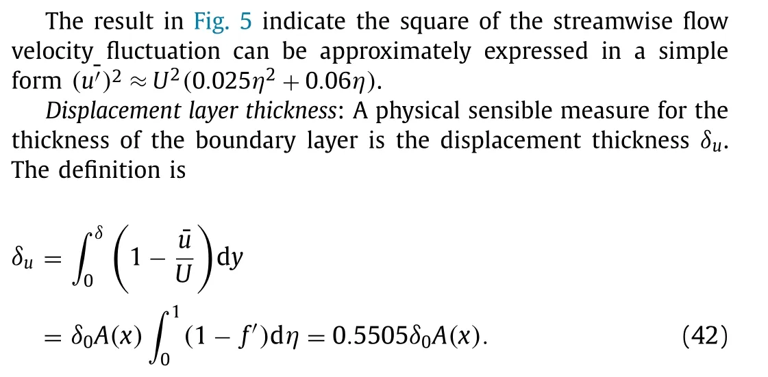
The free stream velocity scales inversely with the boundary layer thickness, the mixing length model could compensate the free stream velocity, so that turbulent boundary layer flow’s partial differential eqiations would be transformed to an ordinary differential equation in a similar way as that for the Blasius similarity equation [2] . Within the frame of the Prandtl mixing length modelling,the similarity solutions that are called as special exact solutions by Schlichting [4] and all related quantities of the 2D turbulent boundary layers are obtained. This study may help facilitate a better understanding of turbulence phenomena.

Declaration of Competing Interest

The authors declare that they have no known competing financial interests or personal relationships that could have appeared to influence the work reported in this paper.

Acknowledgement

This work was supported by Xi’an University of Architecture and Technology (Grant no. 002/2040221134 ). The author wishes to express his appreciation to the anonymous reviewers for his/her high level comments.

Appendix: A complete maple code

restart; with(student); with(plots); beta : = 1; kappa : = 0.4; lambda : = 1; ode : = diff(f(xi), xi, xi, xi) + beta*(1 - diff(f(xi), xi))*(1- diff(f(xi), xi)) + kappa*kappa*diff(xi*xi*abs(diff(f(xi), xi, xi))*diff(f(xi), xi, xi), xi) = 0; sol : = dsolve(ode, f(0) = 0, D(f)(0) = 0,D(f)(lambda) = 1, numeric, output = listprocedure); p0 : = plots:-odeplot(sol, [xi, f(xi)], xi = 0. lambda, color = black, linestyle = [1],thickness = 3, legend = [f(xi)], axes = boxed); p1 : = plots:-odeplot(sol, [xi, diff(f(xi), xi)], xi = 0. lambda, color = blue, linestyle = [2],thickness = 3, legend = [“df/dxi”], axes = boxed); p2 : = plots:-odeplot(sol, [xi, diff(f(xi), xi, xi)], xi = 0. lambda, color = red, linestyle = [3],thickness = 3, legend = [“d(df/dxi;)/dxi”], axes = boxed); u : = plots:-odeplot(sol, [xi, diff(f(xi), xi)], xi = 0. lambda, color = red,linestyle = [1], thickness = 3, legend = [“df/dxi”], axes = boxed); v : = plots:-odeplot(sol, [xi, xi*diff(f(xi), xi)], xi = 0. lambda, color = blue,linestyle = [3], thickness = 3, legend = [“xi;df/dxi”], axes = boxed); plots:-display([p0, p1, p2], axes = boxed); plots:-display([u, v],axes = boxed);