Characterizing human driver characteristics using an artificial neural network and a theoretical model

Sangmyoeng Kim·Takeshi Miyamoto·Tatsuya Kuboyama·Yasuo Moriyoshi

Abstract Human drivers seem to have different characteristics，so different drivers often yield different results from the same driving mode tests with identical vehicles and same chassis dynamometer. However， drivers with different experiences often yield similar results under the same driving conditions.If the features of human drivers are known，the control inputs to each driver，including warnings，will be customized to optimize each man-machine vehicle system.Therefore，it is crucial to determine how to characterize human drivers quantitatively.This study proposes a method to estimate the parameters of a theoretical model of human drivers.The method uses an artificial neural network(ANN)model and a numerical procedure to interpret the identified ANN models theoretically.Our approach involves the following process.First，we specify each ANN driver model through chassis dynamometer tests performed by each human driver and vehicle.Subsequently，we obtain the parameters of a theoretical driver model using the ANN model for the corresponding driver.Specifically，we simulate the driver’s behaviors using the identified ANN models with controlled inputs.Finally，we estimate the theoretical driver model parameters using the numerical simulation results. A proportional-integral-differential (PID) control model is used as the theoretical model.The results of the parameter estimation indicate that the PID driver model parameter combination can characterize human drivers.Moreover，the results suggest that vehicular factors influence the parameter combinations of human drivers.

Keywords Neural network·Identification·Driver model·Chassis dynamometer·Driver characteristics

1 Introduction

Ingeneral，drivingtestsareconductedinachassisdynamometer to evaluate the fuel consumption of passenger cars and emission levels.In addition，engineers use such tests to verify the performance of vehicles under development. To reduce the human efforts and data variations， current researchers focus on robot drivers on chassis dynamometers [1-6]. On the other hand， the driving tests by human drivers are still necessary， and after releasing the cars， human drivers will drive those vehicles on real roads.As human drivers apparently have different characteristics， the drivers often yield different results from the same driving mode tests with identical vehicles on the same chassis dynamometer. However，drivers with different experiences often yield similar results under the same driving conditions.If the features of human drivers are known，the control inputs to each driver，including warnings，will be customized to optimize each man-machine vehicle system.Hence，we are interested in determining how to characterize human drivers quantitatively.For the human drivers’ characterization， it is necessary to develop human driver models，and recently，artificial neural network(ANN)technologies have been very beneficial for such model developments.

Many studies have been conducted on ANN-based driver models[7-10]，ANN-based tuning of proportional-integraldifferential(PID)control [11-14]，and ANN-based characterization of drivers’behaviors[15-22].ANN has also been used to investigate the vehicle speed of robot drivers[7]as well as to build vehicle following and lane change models[8-10]. In addition， methods have been developed to identify the constants of the PID model from ANN [11] and to couple the PID controller with ANN [12-14]. The input of some ANN models are smartphone acceleration signals[15，16]，data acquired on a driving simulator[17]，and vehicleCAN-signalsobtainedwhiledriving[18-20].Onthebasis of the studies above， drivers’ characteristics can be categorized into three types: aggressive， mild， and moderate. In some studies， workload was set as drivers’ characteristics，ANN was constructed using physiological signals as inputs for on-road driving[21]，and drivers were classified according to operation data on a driving simulator[22].However，these studies neither analyzed human drivers’ characteristics quantitatively nor related the ANN driver models to any theoretical driver models.

The rational interpretation such as ANN models is difficult， because the number of weighted factors and biases as their model parameters is too large to achieve a feasible connection for the human behavior mechanism. Therefore，we have been developing a procedure to approximate the identified ANN model to a theoretical model that expresses the mechanism of human drivers’behaviors.If that approximation is realized， we would be able to interpret the characteristics of the ANN driver model from the theoretical one. This achievement would make it possible to characterize individual human drivers using the theoretical model parameters.Here，we use a PID-type theoretical driver model as the theoretical driver model to characterize human drivers on the accelerator pedal operation. We expect that this study will contribute to the research on the characterization of human drivers according to behavior mechanism.Aside factors related to human operation， factors such as engine braking and regenerative braking affect a brake pedal.Therefore， the brake pedal operation was not considered in this study，but will be analyzed in a future study.

The rest of this paper is organized as follows. Section2 describes the experimental setup and model construction conditions.Section3 describes the methods for model construction and calculation of model constants.Section4 illustrates and discusses the results of each model constant，and Sect.5 summarizes the work.

2 Experimental

2.1 Experimental apparatus

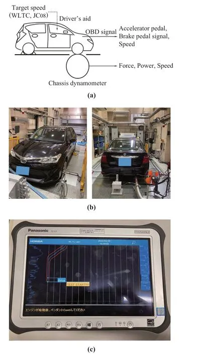
Fig.1 Schematic of the measuring systems.a Schematic of the vehicle.b Installation in the chassis dynamometer.c Driver’s aid

A chassis dynamometer(Horiba，Vulcan)was used to obtain driving data for training the ANN driver model. Two gasoline vehicles(V1，V2)and a plug-in hybrid vehicle(V3)were used as the test vehicles.Figure1a，b shows a schematic of the chassis dynamometer and its installation in the vehicle，respectively.Adriver’said，asshowninFig.1c，wasused.The test drivers accelerated and braked to match the speed pattern of the vehicles with the target speed(±2km/h of the limits).Table1 lists the specifications of each vehicle，while Table2 lists the specifications of the measuring devices.Signals for the ANN driver model were obtained from DST-i (Denso，Japan) for gasoline vehicles and CANedge (CSS Electronics， Denmark) for plug-in hybrid vehicles. The accelerator pedal position，brake signal，and vehicle speed signals wererecorded.The obtained signals of the controller area network(CAN)were synchronized with the vehicle speed on the chassis dynamometer.The sampling period of the data was set to 10Hz.

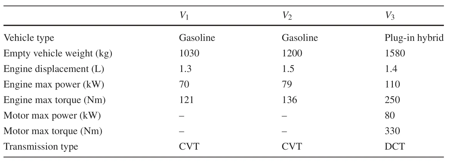
Table 1 Specifications of the vehicles used in the experiments

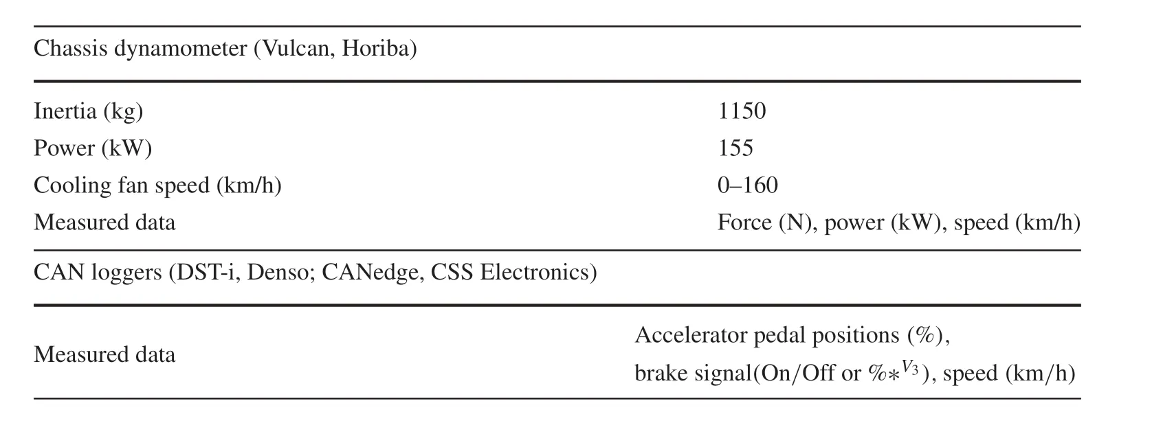
Table 2 Specifications of the measuring systems

2.2 Combination of driving mode，vehicles，and drivers

Worldwide harmonized Light duty Test Cycle (WLTC)， a mode regulated by Worldwide harmonized Light duty Test Procedure(WLTP)，was selected as a learning task.In addition， the driving mode JC08， regulated in Japan by [23]，was selected for testing.An extra high phase of WLTC was not included in Japanese regulations，because the maximum speedlimitonmotorwaysis100km/h.Thevehiclespeedprofiles for each driving mode are shown in Fig.2.TheV3has three modes:EV，HEV，and Power mode.Since the EV mode was possible by pre-charging the battery，data were obtained in EV mode，where the vehicle ran only on a motor.Moreover，data were obtained in HEV mode，where an engine and motor ran simultaneously.Table3 lists the number of modes，drivers，and vehicles.The test execution，order，and distance error are detailed in Table6 of the Appendix.

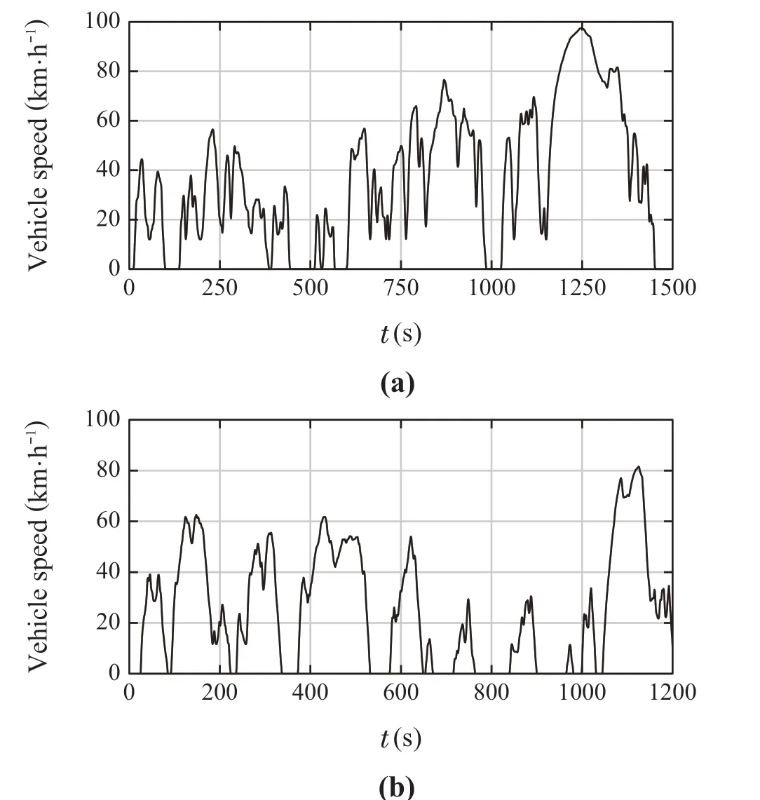
Fig.2 Speed profile of WLTC and JC08.a WLTC.b JC08

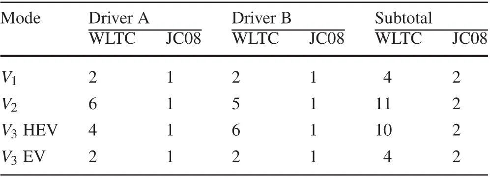
Table 3 Experimental conditions (number of times) for the driving modes and drivers

3 Numerical method relating the ANN driver model to theoretical model

3.1 Overview of the numerical method

First， the dataset was created from the data obtained in the previous section.Subsequently，the ANN driver and theoreticalmodelswereidentified，asshowninFig.3.Theaccelerator pedal was operated by the drivers according to the target speed， and the vehicles were driven considering the speed and acceleration. The ANN driver model was constructed from the data obtained experimentally， and each constant was identified from the theoretical model for the same input.Finally，the model was tested to determine whether the identified constants would exhibit the characteristics of the drivers.

3.2 Construction of the ANN driver model

The structure of the ANN driver model is shown in the top left side of Fig.3.The model specifications are listed in Table4.The developed ANN considered four inputs:vehicle speed，acceleration，the difference between the target vehicle speed and the vehicle speed(P gain)，and the difference between the target acceleration and the acceleration(D gain).The accelerator and brake pedals operation for driving the vehicles were the outputs. As measurements other thanV3acquired only on/off signal from the brake pedal but not brake opening degree or brake pressure，this study focused on the output change of the accelerator pedal opening.A hidden layer was fixed to one layer and the number of the perceptron to 100.The activation function of the hidden layer was set to ReLU，and the function of the output layer was set to linear. The Nadam optimization algorithm was implemented [24]， and the loss function was the root-mean-square error(RMSE)，as in Eq.(1).If the loss function did not change 50 times under 10，000 epochs，the learning process was set to stop

whereyMeasurementisthemeasuredacceleratorpedalopening，yPredictionis the predicted accelerator pedal opening in the ANN driver model，andnis the total number of data.

3.3 Relation of the ANN model to the theoretical model

The theoretical driver model we used to analyze the characteristics of the ANN driver model relied on the following PID-type control model. In this case， the integral gain was omitted， because pre-computational results showed that ithad a negligible effect on the output

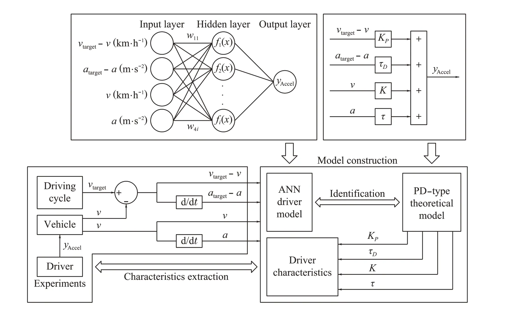
Fig.3 Overview of the ANN and theoretical driver models

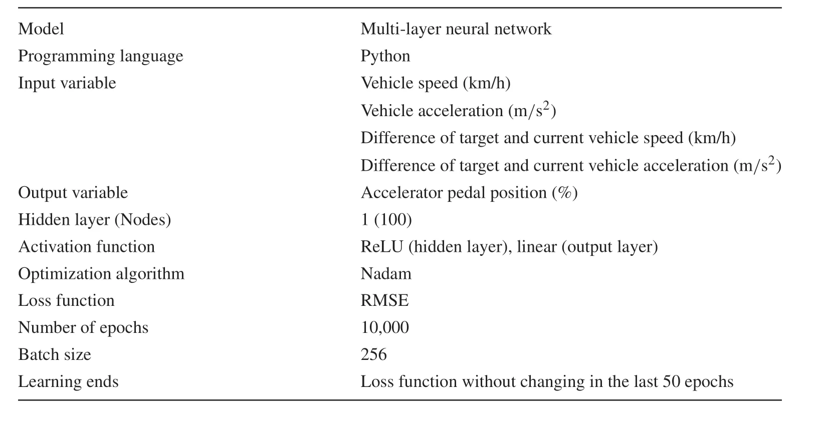
Table 4 Specification of the ANN driver model

whereyAccelis the predicted accelerator pedal opening in the ANN driver model;K PandτDdenote the proportional and differential gains of drivers，respectively;Kandτdenote the proportional and differential gains of the vehicles， respectively;vPis the difference between the target and current speeds;andaDis the difference between the target and current accelerations. Here， a numerical method was used to relate this theoretical driver model to the trained ANN driver model.A method for calculating each gain is defined as follows(5)-(8):

Stay with me; I will give you everything you desire, and I will establish a city here for you, and will furnish it with every requisite147; I will give you the land of the Caucasus, and will make its princes subject to you

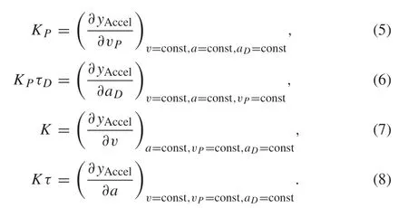
In Eqs.(5)-(8)，each gain(K P，τD，K，andτ)should be a continuous function of the four variables (vP，aD，v， anda).The numerical approach that we developed to obtain the gains is as follows:

(1) Select the values of each variable，so that they appear in the driving mode tests，and choose one typical value of each variable.

(2) Produce the data of the accelerator pedal position using the identified ANN model with controlled input variables for a target variable， keeping the other three variables constant.Use the selected values in step(1).

(3) Plot the accelerator pedal data as a function of the target variable，considering the remaining input parameters as constants.

(4) Calculate the gradient as the gain around a typical value of the target variable using linear approximation.

(5) Repeat steps(1)to(4)for each typical value of the target variable and the other three variables.

The above method makes it possible to obtain all gains at selected discrete points. In step (4)， as the first step of the study，we calculate the gain at limited points to obtain typical gains of the model.The gain calculation results include the same condition and some additional ones to observe the influence of other variables on a target gain.The calculation conditions are realized by treating the variables as controlled inputs of the identified ANN model.

Table5 shows an example of the fixed values for vehicle speed，acceleration，vP，andaDfor the four inputs.Cases 1 to 8 considered constant vehicle speeds with varying accelerations and constant accelerations with varying speed.The variables in the table are listed for a practical range， which is the same as that used to calculate the gain presented above.For example，to findK Pin case 1，fixv= 20km/h，a= 0m/s2， andaD= 0.25 m/s2， and only vary the value ofvPfrom-1.5 to+1.5km/h.Figure4 illustrates a partial result of the ANN driver model built with the WLTC data of driver A.Only the value of the vehicle speed difference(vP)was varied to obtain the value numerically among the inputsto the trained ANN driver model.For the input of the ANN driver model，the accelerator pedal opening(yAccel)was considered the output.The slope was used to obtain theK Pgain.Similarly，the range for varying thev，a，andaDinputs was 0km/h to 90km/h，-1.5m/s2to+1.5m/s2，and-0.5m/s2to+0.5m/s2，respectively.This range includes 95%of the total number of datapoints for eachvalue.Followingthesameprocedure，K，τ，K P，andτDcould be obtained from Eqs.(5)to(8). Other calculations were performed under different calculation conditions forvPandaDas shown in Appendix B.

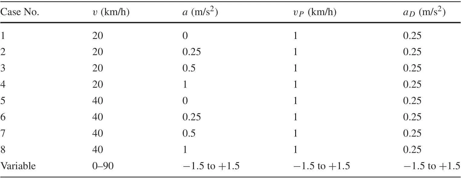
Table 5 Selected constants of v，a，vP，and aD as input data for identified ANN driver models

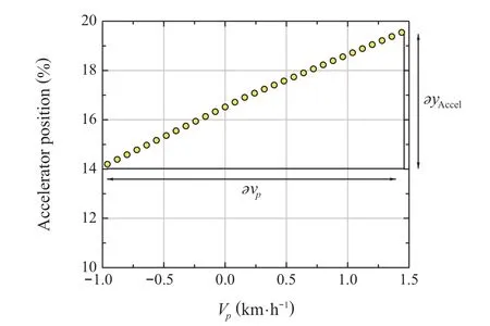
Fig.4 Example of extraction of K P gain under the ANN driver model for driver A

4 Results and discussion

4.1 Learning and testing the ANN driver model

Figure5 shows the RMSE values for the ANN driver model learning results for each driver and vehicle using the four inputs.In the case of learning WLTC and testing WLTC，the accuracy of the RMSE was less than 5%in all cases.When learning WLTC was tested using the JC08 data，the prediction accuracy ofV3reduced for driver B.Figure6 shows the testing results of WLTC for drivers A and B，while Fig.7 depicts the results of testing JC08 for drivers A and B.The left side of Figs.6 and 7 shows the time-series results of the experiment and prediction， whereas the right side of both figures compares the values of the experiment and prediction in a distribution plot.As mentioned above，the learning was considered successful when the RMSE was low.The results were consistent with the experimental values.However，when the RMSE was high，the accuracy of the accelerator pedal prediction deteriorated.A reason for these results is that，as shown in Appendix A， the JC08 data used for the test of Driver B were measured in the latter half of the tests when Driver B was more adapted to the experiment. Thus， the learning process could not have been adequately achieved， because learning with the WLTC data from a driver not familiar with the driving test and then testing the JC08 data with a driver accustomed to driving could have resulted in biased results.Therefore，in this study，learning decisions were considered successful when the RMSE accuracy was less than 5%.The gain using the ANN driver model in the case of testing with WLTC was analyzed.

4.2 Characteristics of drivers for different vehicles

Figure8 shows the results ofK，τ，K P，andτDof the learned ANN driver model for each driver regarding the effects of the acceleration (0， 0.25， 0.5， 1 m/s2) and speed (20， 40 km/h)conditions listed in Table 5.The results ofV1，V2，V3HEV，andV3EV are shown in Fig. 8a， b， Fig. 8c， d， Fig. 8e， f，and Fig. 8g， h， respectively. Each point corresponds to the average values processed for each test from cases 1 to 8，as described in Table5.For example，the points with acceleration and vehicle speed of 0m/s2and 20km/h(black square in the figure)represent case 1.The differences inKandK Pbetween filled and unfilled cases are also shown in the figures.As the gains obtained from the ANN driver model areKτandK PτD， the values ofτandτDwere obtained by dividing each gain intoKandK P，respectively.

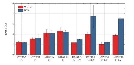
Fig.5 Reproduction and prediction accuracy of the ANN driver model

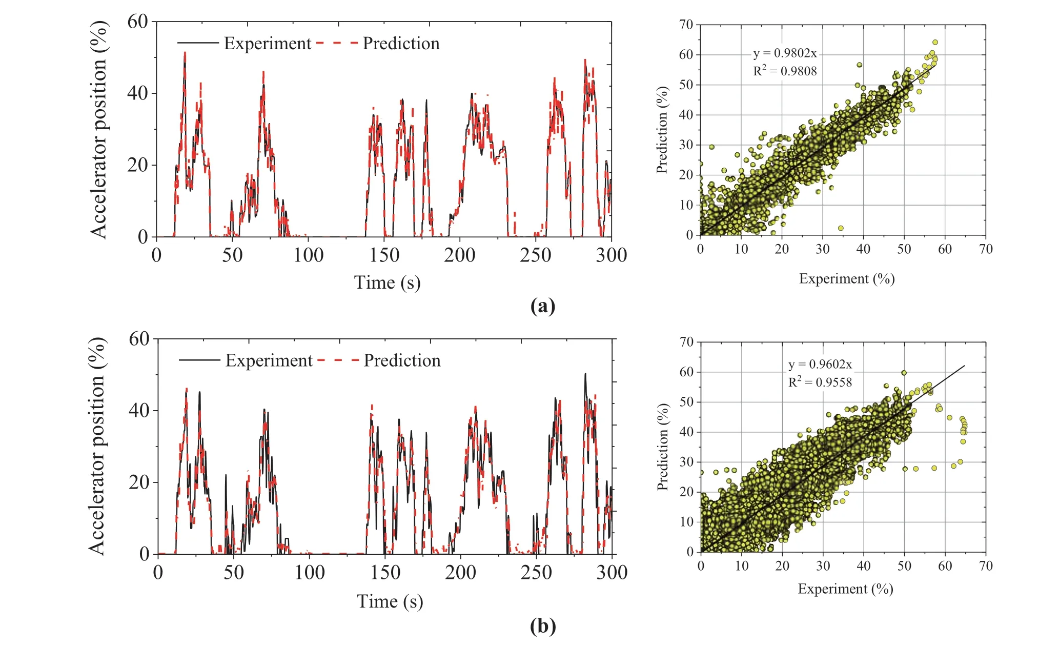
Fig.6 Accuracy of the developed ANN driver model(learning WLTC and testing WLTC).a Driver A(left:time series;right:scatter experiment and prediction).b Driver B(left:time series;right:scatter experiment and prediction)

For the case ofKandK Pshown in Fig.8a， c， e， g， the gainKdepending on the speed of each vehicle ranges from 0.1 to 1 for the vehicle speed itself.In contrast，the gainK Pdepending on the speed difference controlled by the driver ranges from 1 to 10. For the case ofKandK Pshown in Fig.8b，d，f，h，τdue to acceleration for each vehicle ranges from 10 to 100.In addition，τD，which applies to the acceleration difference controlled by the driver，ranges from 0.1 to 10.Previous studies showed that theK Pgain was from 0.4 to 10，whileτDwas from 0.4 to 1[4-6].Although some parts exist whereK Pis small andτDis large，various conditions show a trend towardK P ＞Kandτ ＞τD. Note thatK Pbeing larger thanKmight be due to the driver’s perception of the speed difference rather than the gain related to the speed of the vehicle itself.The smaller the timescale valueτD，the more frequently the driver adjusts the vehicle while operating the accelerator pedal.In other words，gainsK PandτDare more important driving characteristics thanKandτ.

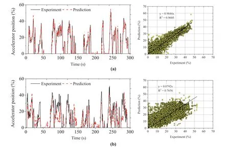
Fig.7 Prediction accuracy of the developed ANN driver model (learning WLTC and testing JC08). a Driver A (left: time series; right: scatter experiment and prediction).b Driver B(left:time series;right:scatter experiment and prediction)

When considering driver A and evaluating the values ofKandK Pdepending onV1toV3，the value ofKis almost as low as 0.2 to 1.0， whereas the value ofK Pvaries from 0.2 to 5.6. When considering driver A and focusing onτandτDwithV1toV3，τshows high values from 9.4 to 43.2，whereas the value ofτDvaries from 0.2 to 3.0. Although driver B has a larger timescale than that of driver A， the range ofKandK P，and the values ofτandτD，show similar trends.As mentioned above，Kandτare lower effects thanK PandτD.In real driving situations，the drivers’behavior depended on the conditions of the vehicle distances between the frontal and later vehicles [25]. However， when human drivers drive on the chassis dynamometer， they drive by adjusting the difference between the target vehicle speed and current speed.In this case，quantitative differences were presented in the gains calculated using the data from the ANN driver model.

4.3 Characterization of drivers in gain and timescale plane

As mentioned above，the vehicle speed and acceleration substantially affect the driver’s maneuver on the target speed and acceleration.Moreover，Kandτwere compared as the characteristics of each vehicle， as shown in Fig. 9. In contrast，Fig. 10 depicts the comparison ofK PandτDas the characteristics of the driver.Each point results from learning the test conditions described in Table 3 and plotting all the results obtained from the calculation conditions listed in Table 5.In Fig.9，theKgains show differences due to the vehicle speeds of 20km/h(square mark in Fig.9)and 40km/h(round mark in Fig.9).Nevertheless，the differences due to the driver are not evident，resulting in an overlap ofKandτ.InV1andV3HEV， driver A tends to have a highK Pand lowτD， while Driver B tends to have a lowK Pand highτD.InV3EV，the trend is similar;however，a difference between the upper and the lower values is present. InV2， the distributions ofK PandτDof drivers A and B are similar.It is thought that the larger theK Pgain due to the speed difference， the earlier the accelerator pedal is operated， and thus， the smaller the timescaleτDgain becomes.A driver’s attitudes，experience，workload，and age may influence the driver’s behavior when operating the acceleration and brake pedal[25-28].The differences in each gain distribution are shown in Fig.10.The error distance difference is about 1.18%±0.39%from 75 to 390m for a total distance of 15 km to track a speed profile with a limitation such as mode driving. Despite such small differences in distance，the model constants differ by drivers.The results shown in Fig.10 indicate that individual human drivers can be quantitatively characterized by the estimated values ofK PandτDgain. More data will be required for analysis in the future to clarify the relationship among the estimated gain values ofK PandτD，the human drivers，and fuel consumption.

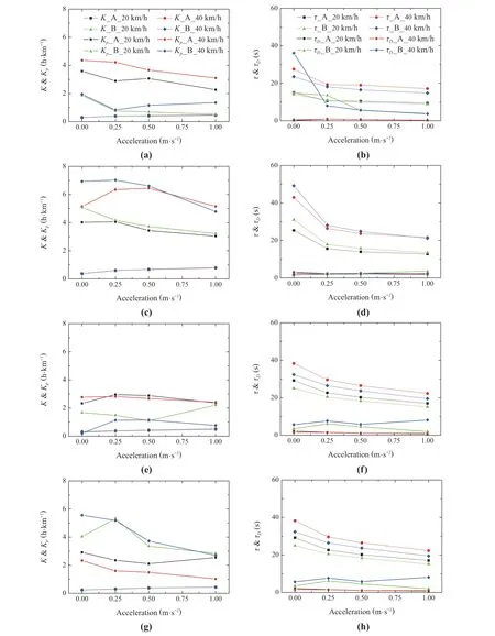
Fig.8 Comparison of the gains(K， K P，τ，τD)for various vehicles.a K and K P of V1.b τ and τD of V1.c K and K P of V2.d τ and τD of V2.e K and K P of V3 HEV.f τ and τD of V3 HEV.g K and K P of V3 EV.h τ and τD of V3 EV

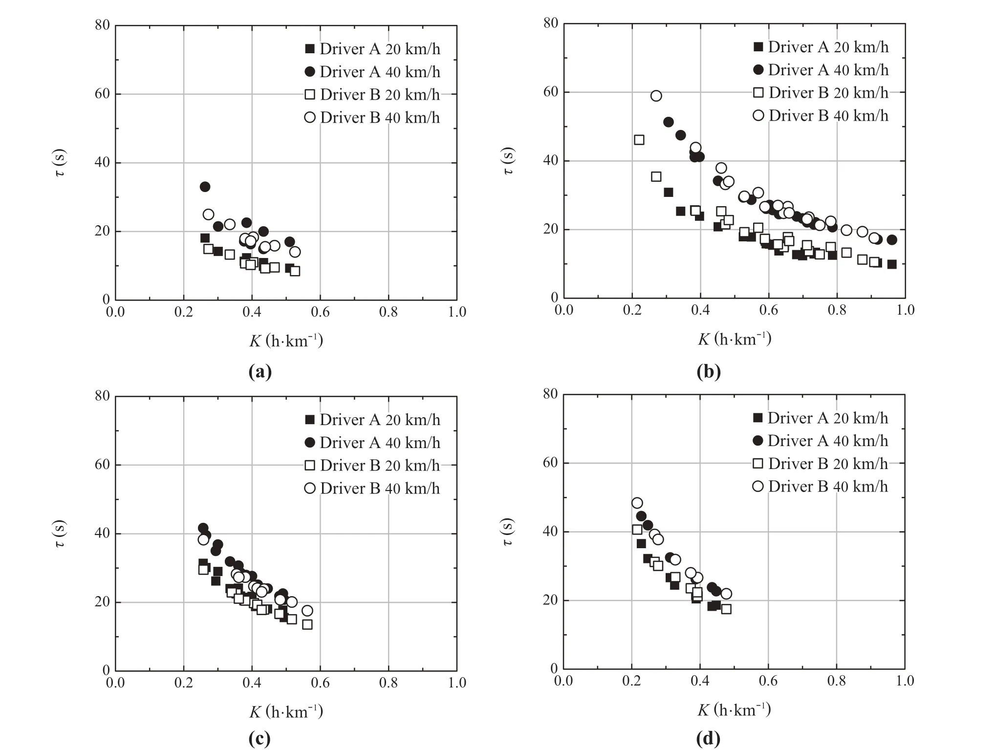
Fig.9 Estimated K and τ gains for each driver and vehicle.a V1.b V2.c V3 HEV.d V3 EV

5 Summary

This paper introduces a method for estimating the model parameters of a PID-type theoretical driver model from the identified ANN driver model to define the characteristics of human drivers. At first， ANN driver models for vehicle acceleration pedal operation are identified using chassis dynamometer tests performed by two human drivers with four vehicle types. Next， the driver’s acceleration pedals operations are numerically simulated using those identified ANN models with controlled inputs such as vehicle speed，acceleration，and differences between target and current values in terms of speed and accelerations.Finally，the theoretical driver model parameters are estimated based on the numerical simulation results. The results indicate the following. First， combinations of the proportional gainK Pof the velocity difference and timescale of the acceleration differenceτDcan characterize drivers’ behaviors in terms of acceleration pedal operation even for the driving modes where very slight differences in the resulted driving distances between two drivers.The three of four vehicle types exhibited noticeable differences in driver characteristics between the two drivers.Second，the vehicle characteristics influenceK PandτD.Further data acquisition and analysis are needed to understand the parameters that can characterize human drivers related to vehicle and driving conditions.

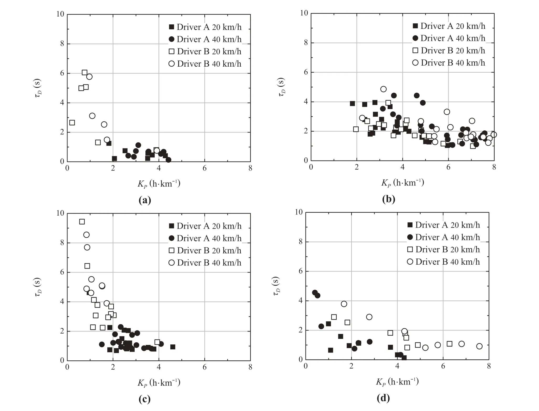
Fig.10 Estimated K P and τD gains for each driver and vehicle.a V1.b V2.c V3 HEV.d V3 EV

AcknowledgementsThis work was the result of a collaborative research program with the Research Association of Automotive Internal Combustion Engines(AICE)for the fiscal year 2020.The authors gratefully acknowledge the concerned personnel.

Appendix A: Experimental history information

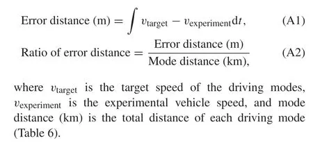
Appendix B:Additional simulation results

We have performed additionalK PandτDestimations under thevPandaDconditions different from those presented in Tables 7 and8. The results are illustrated in Figs.11， 12，13 and 14. A similar trend was observed in the results， as illustrated in Figs.9 and 10. Differences inKandτwere observed depending on the vehicle speed conditions，whereas the trends ofK PandτDdepended on the drivers.

All theK PandτDestimation results in this paper indicate that the tested drivers have differentK P-τDcombinations for the three vehicles.In particular，the results for HEV and EV show that the drivers’K PandτDdata are plotted in different regions in theK P-τDplanes for each driver under all the driving conditions，i.e.，all the combinations of the values ofv，a，vP，andaD.In addition to that，theV1drivers’plotted data regions in theK P-τDplane show a similar tendency except for the conditions including the smallestvP，andaDvalues. In the case of the smallestvPandaDcombination，since the influence of the difference between the current and targetvaluesissmall，thedifferenceinthedrivers’parameters may not be so significant. On the other hand， the results in terms ofV2show that the tested drivers have almost the same plotted data regions. The vehicle characteristics may cause this.

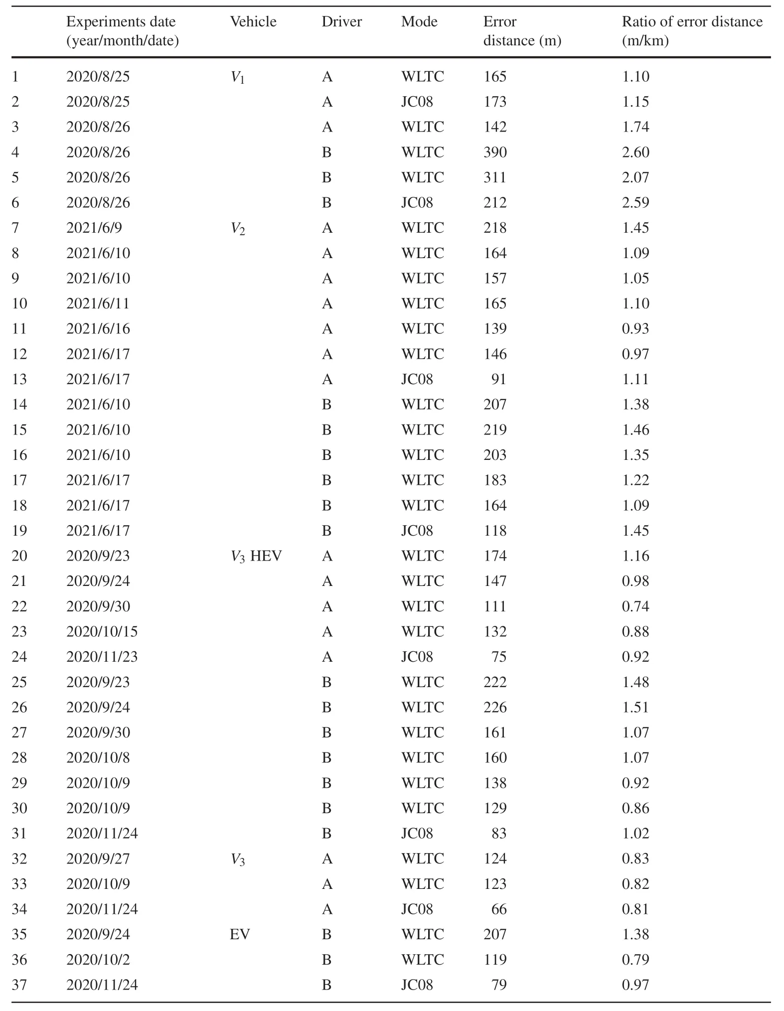
Table 6 Experimental history information

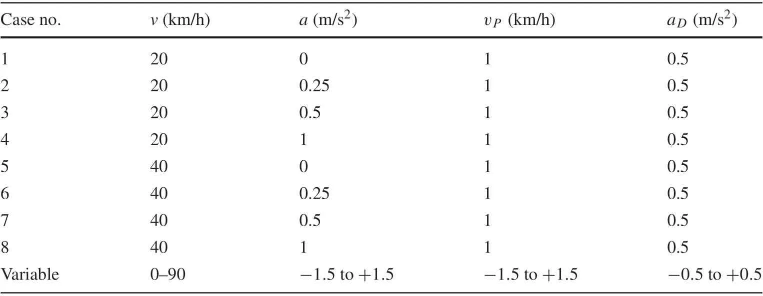
Table 8 Selected constants of v，a，vP，and aD as input data for identified ANN driver models(2)

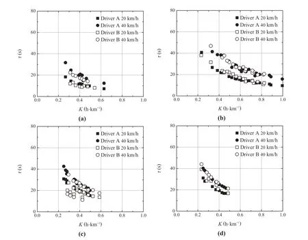
Fig.11 Estimated K and τ gains for each driver and vehicle(Condition Table 7).a V1.b V2.c V3 HEV.d V3 EV

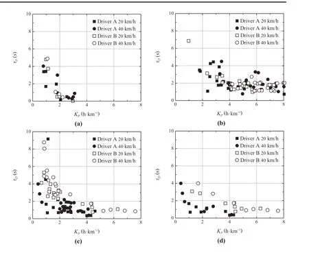
Fig.12 Estimated K P and τD gains for each driver and vehicle(Condition Table 7).a V1.b V2.c V3 HEV.d V3 EV

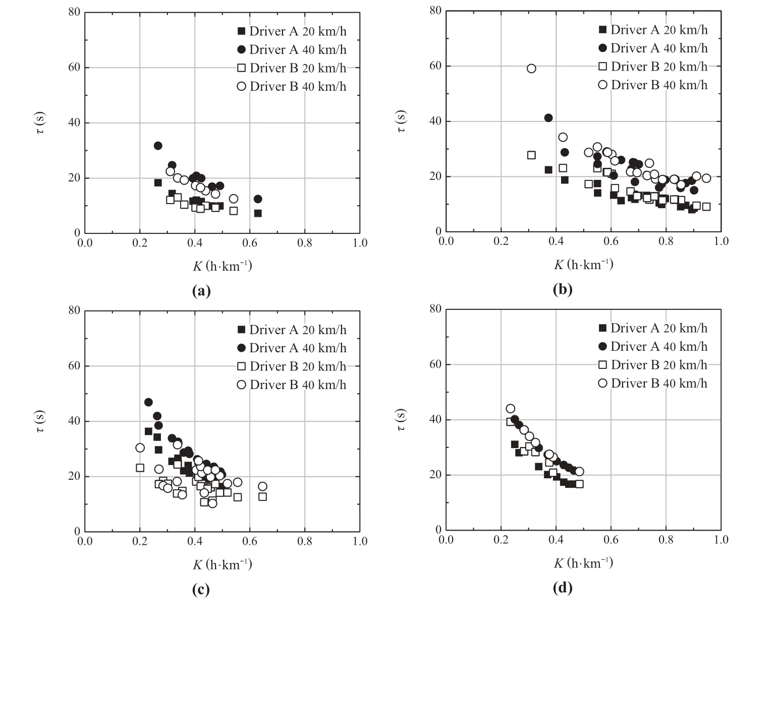
Fig.13 Estimated K and τ gains for each driver and vehicle(Condition Table 8).a V1.b V2.c V3 HEV.d V3 EV

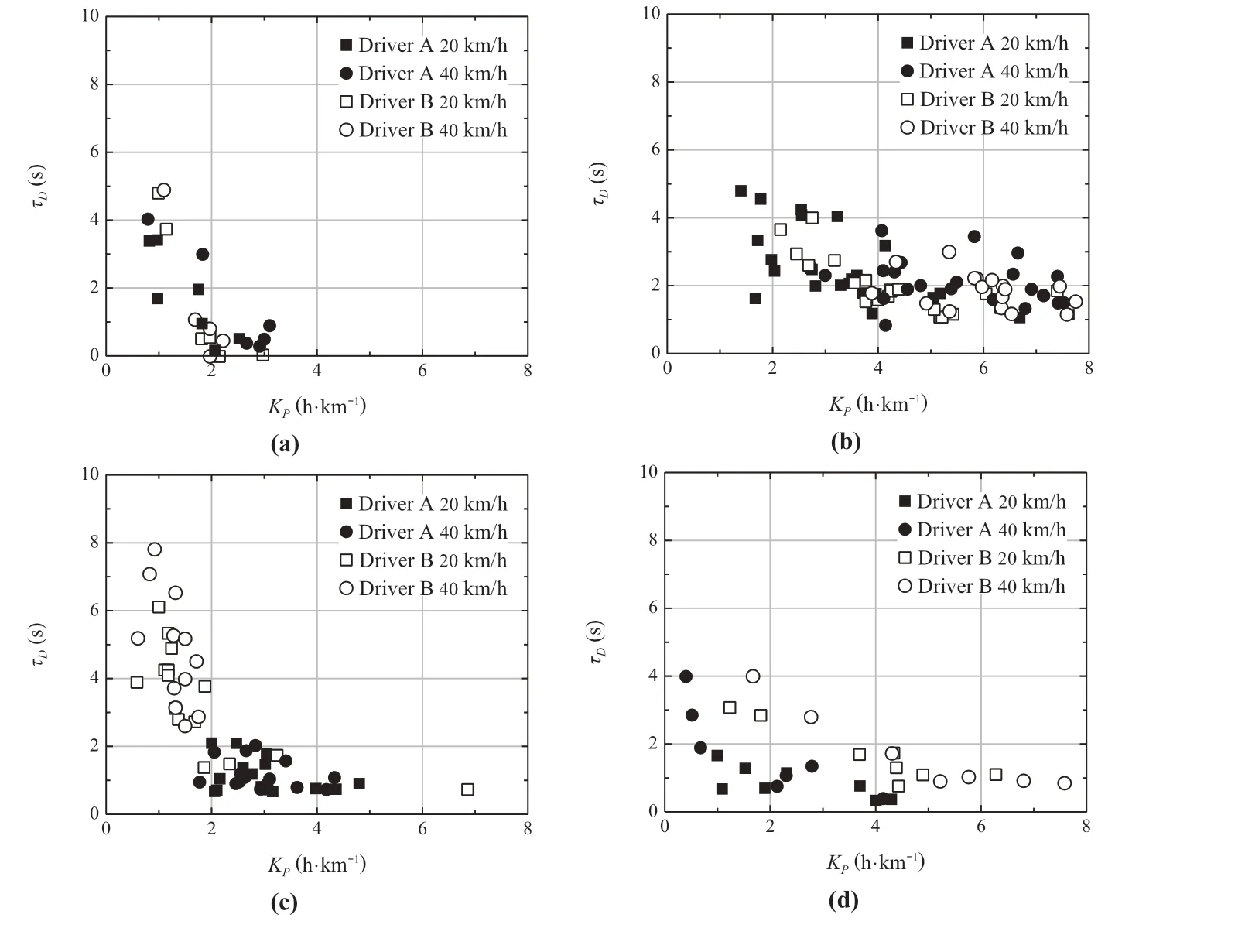
Fig.14 Estimated K P and τD gains for each driver and vehicle(Condition Table 8).a V1.b V2.c V3 HEV.d V3 EV