Probability-based analytical model for predicting the post-earthquake residual deformation of SDOF systems

Zhang Qin , Gong Susu, Gong Jinxin, Zhang Guanhua and Xi Guangheng

1. College of Civil and Transportation Engineering, Hohai University, Nanjing 210098, China

2. Highway Maintenance Technology Research and Development Center of Liaoning Provincial Communication Planning & Design Insitute Co. Ltd., Shenyang 110111, China

3. Department of Civil Engineering, Dalian University of Technology, Dalian 116014, China

Abstract: A probability-based analytical model for predicting the seismic residual deformation of bilinear single-degreeof-freedom (SDOF) systems with a kinematic/Takeda hysteretic model is proposed based on a statistical analysis of the nonlinear time history response, and the proposed model explicitly incorporates the influence of record-to-record variability. In addition, the influence of primary parameters such as the natural vibration period, relative yield force coefficient, stiffness ratio and peak ground acceleration (PGA) on the seismic residual/maximum deformation ratio (dR/dm) are investigated. The results show that significant dispersion of the dR/dm ratio is observed for SDOF systems under different seismic ground motion records, and the dispersion degree is influenced by the model parameters and record-to-record variability. The statistical distribution of the dR/dm results of SDOF systems can be described by a lognormal distribution. Finally, a case study for seismic residual deformation and reparability assessment of the bridge structure designed with a single pier is carried out to illustrate the detailed analytical procedure of the probability-based analytical model proposed in this study.

Keywords: residual deformation; probability model; repairability assessment; single-degree-of-freedom system; nonlinear seismic response; record-to-record variability

1 Introduction

Post-earthquake reconnaissance indicates that seismic losses are triggered not only by building collapse but also by structural rehabilitation and rebuilding after an earthquake, and the cost for repairing and rebuilding damaged structures could be enormous (Hsu and Fu, 2004; Decaniniet al., 2004; Hashimotoet al., 2005; Zhanget al., 2017). Therefore, there are some limitations of the traditional performance assessment method based on the maximum deformation, which is the key index in determining the collapse-resisting capacity of structures. The indexes of the collapse resistance capacity and repairability both need to be emphasized in newly proposed performance-based seismic design philosophy of structures; that is, both the maximum deformation and residual deformation play key roles in determining the properties of structures subjected to seismic excitation (Leeet al., 2010; Hatzigeorgiouet al., 2011; Saidiet al., 2012). It is well known that a number of damaged RC columns and structures have to be demolished due to the large residual deformations that arise in the aftermath of many earthquake events, such as the Michoacan earthquake in 1985 (Rosenblueth and Meli, 1986), the Kobe earthquake in 1995 (Fujinoet al., 2005) and the Wenchuan earthquake in 2008 (Hanet al., 2013; Zhanget al., 2017). Therefore, the limitations of traditional performance assessment methods based on the maximum deformation must be addressed, and a more reasonable method based on both the maximum deformation and residual deformation should be provided.

To evaluate the residual deformation, extensive research has been conducted from a practical perspective. MacRaeet al.(1997) and Kawashimaet al.(1998) studied the post-earthquake residual deformation of bilinear single-degree-of-freedom (SDOF) systems with given displacement ductility demands based on the results of nonlinear time history analysis. They defined the residual deformation response spectrum (rR) as the ratio of the residual deformation to maximum possible residual deformation with variations in a stiffness ratio to predict the residual deformations of bilinear SDOF systems. In their studies, the trend of residual deformation with variation in natural vibration period was not clearly identified, and the influence of seismic level, recordto-record variability and maximum deformation (i.e., ductility ratio) were neglected. However, Ruiz-Garciaet al. (2006) showed that the residual deformation of a SDOF system is not only affected by the stiffness ratio but also strongly dependent on the seismic levels, record-to-record variability, natural vibration period in the short period region (e.g., 0.5T< s), lateral strength ratios and types of hysteretic behavior. Guerreroet al. (2017) studied the residual displacement demands of SDOF systems subjected to earthquake ground motions recorded at soft soil sites of Mexico City, and also found that the significant parameters affecting residual displacements are stiffness ratio, hysteretic response, ductility level and so on. Their research also highlighted that the dispersion is very high in predicting residual displacement demands for SDOF systems subjected to earthquake ground motions recorded in soft soil sites and in firm soil sites. In addition, Pampaninet al. (2003) and Christopouloset al. (2003, 2004) studied the residual deformation of SDOF and multiple-degree-of-freedom (MDOF) systems through time history analyses and indicated that the hysteretic characteristics, post-yielding stiffness, intensity of the seismic input, and maximum ductility greatly influenced the residual deformations. Considering the influence of the main parameters mentioned above, some different empirical models for predicting the residual deformation response of SDOF systems have been investigated by several researchers, including Gonget al. (2011), Haoet al. (2013) and Huet al. (2015). Although these models were established for simplicity and practical application, the uncertainty in estimating residual deformations induced by recordto-record variability and structural parameters are ignored, and the prediction results may be inconsistent with actual situations. In view of this, Ruiz-Garcia and Miranda (2010) proposed a probabilistic procedure for computing residual deformation demand for multistory regular frame structures, which considered the uncertainty of record-to-record variability and ground motion intensity. Similarly, a post-earthquake damage assessment model of RC structures considering the residual deformation attained during the earthquake based on Bayesian analysis was presented by Yazgan and Dazio (2011). Recently, studies on the uncertainty and probabilistic models of residual deformations have received more attention from researchers. Daiet al. (2017) employed the probabilistic approach to establish the relationship between the maximum deformation and residual deformation of the buildings to consider the uncertainties of the model error dispersion and record-torecord variability. Guo and Christopoulos (2018) studied the probabilistic distribution of the ratio of residual and peak displacements of idealized SDOF systems with non-degrading behavior and proposed a probabilistic model for predicting the residual deformation of the systems.

From the literature review, note that residual deformation is considered an important design indicator for restorability and is of great concern to many seismic researchers and engineers. However, the existing empirical models of residual deformation primarily depend on deterministic models established based on the mean statistical results of the nonlinear time history response of SDOF systems, and the influence on the uncertainty of record-to-record variability and structural model parameters are usually not considered. Although only a few probabilistic models of residual deformations of SDOF systems have been proposed in previous studies, the existing models are mainly aimed at systems with non-degrading hysteretic behaviors. Obviously, systems with degrading hysteretic behavior are more suitable for characterization of RC structures subjected to cyclic loading, and the residual deformations of these systems should also be studied. In addition, the existing models of residual deformation are generally oriented to systems with a constant-ductility demand (i.e., the displacement ductility demand of the system is known in advance), but in fact the displacement ductility demand of the system, especially for existing structures, is generally unknown, and an appropriate residual deformation model is needed for systems with initial properties (e.g., the period, postyielding stiffness ratio, relative yield force coefficient and so on) that are known in advance. Therefore, the main purpose of this study is to discuss the influence of record-to-record variability and model parameters on the residual deformation of SDOF systems with degrading and non-degrading hysteretic behavior and with initial properties known in advance. A probability-based model incorporating the uncertainty of seismic input records and structural model parameters for estimating the residual deformation is proposed based on the statistical analysis of nonlinear time history results of SDOF systems. Meanwhile, the evaluation of residual deformation and repairability for a bridge structure designed with a single RC pier is taken as an example to illustrate the application of the proposed model in the performancebased seismic assessment methodologies. Note that this study ignores the soil-structure interaction (SSI) effects andP–∆ effects, and the results given herein should be interpreted from this perspective.

2 Nonlinear time history analysis of a SDOF system

2.1 Analytical model

As shown in Fig. 1, a reinforced concrete bridge pier can be equivalent to a SDOF system, and residual displacement (dR) of the structures can be predicted by nonlinear time history analysis of the SDOF system with the given ground motion records. The structural characteristics of the SDOF system are mainly related to the design parameters such as the initial stiffness (ki), the concentrated mass (m) and the period (T). Assuming that the concentrated mass (m) is equal to a unit mass, the natural vibration period of the model can be calculated as follows:

Fig. 2 Bilinear hysteresis models

wherekiis the initial stiffness of the model and defined as the secant stiffness at the yield point.

In this study, two typical bilinear hysteretic models (i.e., the kinematic hysteretic model and the modified Takeda hysteretic model shown in Fig. 2) with different post-yielding stiffnesses were adopted to reasonably reflect the concrete structure characteristics. For convenience, these two hysteretic models are abbreviated as the K-model and T-model, respectively, in the text. For the K-model, the hysteretic behavior of the system is characterized by non-degradation, excellent energy dissipation capacity and no cumulative damage. Therefore, the corresponding unloading stiffnesskuis expressed as the initial stiffnesski(i.e.,ku=ki) of the system. For the T-model, the hysteretic behavior is characterized by stiffness degeneration, pinching effects and an imperfect energy dissipation capacity. Therefore, the unloading stiffness (ku) is expressed asby the initial stiffness (ki) and the displacement ductility coefficient (µ∆) of the system, and the coefficientα′ is related to the unloading stiffness and can be taken as 0.4 (Takeda and Nielsen, 1970). From the above, the T-model can describe the degradation and pinching behaviors well for RC structures subjected to cyclic loading, but the K-model is more efficient and simpler to use in the seismic response analysis of structures (Kawashimaet al., 1998; Gonget al., 2011). Therefore, these two models are adopted in the analysis of residual deformations of SDOF systems in this study.

Fig. 3 Time history analyses of SDOF systems with different hysteretic models

To illustrate the effects of the hysteretic model on the nonlinear seismic response of the structures, a case study of the nonlinear seismic response analysis of SDOF systems with the K-model and T-model under the same ground motion record was conducted by using SAP2000 software. In the case study, the influences of the system period (T) and post-yielding stiffness ratio (r) were also considered. The period was taken as 0.6 s or 1.2 s, and the post-yielding stiffness ratio (r) was taken as 0.05 or 0.1. The El Centro accelerogram listed in Appendix Table A.1 was selected as the ground motion input, and the seismic ground motion was normalized by the peak ground acceleration (PGA) of 0.25 g. Figure 3 presents the nonlinear time history analysis results of different SDOF systems with the K-model and T-model under the same normalized seismic ground motion, and the corresponding time history response curves of these two models are represented by dark lines and light lines, respectively. From the figure, it is noted that the time history response curves of the SDOF systems with the K-model and T-model have significant differences even though the system parameters and ground motion input are the same. Undoubtedly, there is also a difference in the residual deformation (dR) and the maximum deformation (dm) results of the SDOF system determined by the two different hysteresis models, and the degree of difference may be related to the period (T) and stiffness ratio (r). In general, the difference of the residual deformations with these two models is more obvious when the stiffness ratio (r) is small and that of the time history response curve is more obvious when the system period (T) is large. This suggests that the hysteretic properties (or hysteretic models) have different effects on the time history response and residual deformations of SDOF systems with different parameters. Therefore, it is necessary to consider the influence of the hysteretic model in residual deformation predictions. For this purpose, several statistical analyses are conducted in this study to determine the distribution characteristics of the residual/maximum deformation ratio of different SDOF systems with the K-model and T-model.

In view of the above, the influences of the system period (T) and the post-yielding stiffness ratio (r) on the seismic response of the SDOF systems is also considered in this study. The variation range of the period (T) is 0.2–3.0 s, and the values are selected at an increment of 0.2 s. Eight post-yielding stiffness ratios (r), 0.0, 0.01, 0.05, 0.1, 0.15, 0.2, 0.25 and 0.3, are selected for the analysis.

2.2 Selection of earthquake ground motion records

According to the study conducted by Chenget al.(2013), the seismic response of SDOF systems with bilinear hysteresis models is related not only to the system period (T) and post-yielding stiffness ratio (r) but also to the relative yield force coefficient (η) and peak ground acceleration (αpg). Where, the relative yield force coefficient (η) is defined as the ratio of the yield load to gravity load (i.e.,η = Fy/mg), which is to reflect the elastic-plastic capacity of the systems, and the details can be found in research of Chenget al.(2013). To consider the effects of the parameters mentioned, the relative yield force coefficients (η) are assumed to be 0.1, 0.2 and 0.3. and the peak ground accelerations (αpg) are assumed to be 0.2 g, 0.4 g and 0.6 g for normalization of seismic records to simulate the different seismic levels.

Furthermore, a total of 100 strong ground motion records of different seismic events and site conditions were selected from the PEER (Pacific Seismic Engineering Research Center) strong earthquake database as the seismic input of nonlinear time history analysis for considering the influence of record-to-record variability on residual deformations of SDOF systems. According to the previous studies (e.g., Liossatou and Fardis, 2016; Guerreroet al., 2017; Guo and Christopoulos, 2017), the 100 ground motions with a large variation in parameters such as frequency content, duration, site condition and pulse-characteristics were selected because these are key influence parameters for the the residual deformations of the SDOF systems. Of the 100 ground motions, 88 records that were recorded from magnitude 5.3 to 8.1 events at source-to-site distances of less than 20 km, and the remaining records obtained from magnitude 5.8 to 7.5 events at the distances ranging from 20 km to 50 km. Note that this study mainly focus on the influences of randomness and uncertainty of earthquake ground motions on the residual deformations of the SDOF systems triggered comprehensively by these characteristics mentioned above. So, the influences of the earthquake ground motions characterized by a certain variable such as the site condition, duration and so on were not considered specially. The ground motion records parameters are shown in the appendix Table A1.

3 Statistical analysis of the residual deformation of a SDOF system

3.1 Dispersion analysis and parametric study

The requirements of modern seismic design philosophy indicated that not only the capacity of collapse resistance but also repairability should be required for designing structures subjected to strong earthquake excitation. Therefore, the ratioβ(=dR/dm) of the residual deformation to maximum deformation was taken as the statistical parameter in this analysis, and the influences of the model parameters, record-to-record uncertainty, hysteretic models and seismic intensity levels were also considered. The variation trend of the deformation ratio (dR/dm) with the increase in period (T) for the different bilinear SDOF systems under each of the 100 normalized ground motion records is shown in Fig. 4, and the corresponding mean values of deformation ratio (β) with the variation in period (T) are also presented. From Fig. 4, the obvious dispersion of the deformation ratio (β) is observed for SDOF systems with different ground motion records, although the peak ground acceleration is the same, which indicates that the seismic response results of the systems are also significantly affected by the spectrum characteristics and duration of the ground motion records. Certainly, the degree of dispersion is also related to the model parameters such as the hysterical model, stiffness ratio (r) and natural period of vibration (T). The analytical results ofβ(i.e.,dR/dm) of the systems based on the T-model are relatively concentrated because the degrading hysteretic behavior is considered, showing a smaller dispersion than the results of the K-model. The dispersion of analytical results obviously decreases with the increase of the stiffness ratio (r) of the systems. In addition, the influence of the period (T) on the dispersion ofβis also associated with the stiffness ratio (r) and hysteretic model. The dispersion decreases with the increase in period (T) when the stiffness ratio (r) is large, while the dispersion may remain consistent with the increase in period (T) when the stiffness ratio (r) is small. Additionally, the influence trend of the period (T) on the dispersion ofβis relatively prominent when the system is based on the K-model.

Note that the statistical results of the deformation ratio (β) are also affected by the relative yield load factor (η) and the peak ground acceleration (apg). This can be explained by the fact that the seismic residual deformation may occur in the post-yielding response phase, and the yielding of the structures is mainly related to the two parameters mentioned above (i.e.,ηandapg). Therefore, these parameters play an important role in the residual deformation analysis of the SDOF systems. Furthermore, according to the variation trends of the mean values of the residual/maximum deformation ratio (β) with the periods (T) for the SDOF systems shown in Fig. 4, the effects of the hysteretic model, stiffness ratio (r) and period (T) on the seismic response may seem more obvious than those affected by the peak ground acceleration (apg) and the relative yield force coefficient (η).

3.2 Analytical method and statistical parameters

The detailed procedure of the probabilistic model for predicting the residual deformations of SDOF systems in this study is as follows: (1) 100 ground motion records selected from different earthquake events were normalized by the intensity index of the peak ground accelerationapg=0.2 g, 0.4 g, or 0.6 g. Note that the SDOF systems studied herein are given the initial properties (e.g. relative yield force coefficient) in advance, so the yield states of these structures under different seismic levels need to be concerned, which is vital for the study of the residual deformations. The study herein is obviously different from previous studies on the residual deformations of SDOF systems that have a known target ductility demand, which implies that the yield deformation of the system under each seismic ground motion needs to be determined by iteration according to the given target ductility demand (Kawashimaet al., 1998). Therefore, it is reasonable to conduct amplitude normalization for the ground motions using the peak ground acceleration. (2) The deformation ratios (β) of different bilinear SDOF systems under each of the 100 normalized ground motion records was obtained from statistical analyses of the nonlinear time history seismic response. In this study, the determination of the residual deformation of the system by the residual/maximum deformation ratio (β) is based on the premise that the two deformations mentioned above are independent of each other. Although the residual deformation is affected by the maximum deformation, there is no clear correlation between the two, because the system unloads from a post-peak random point instead of the maximum deformation point (see the nonlinear time history analytical results of SDOF systems shown in Fig. 3). Similar results and conclusions have also been drawn in previous studies (e.g., Kawashimaet al., 1998; Guo and Christopoulos, 2018). (3) the statistical parameters (i.e., mean value and coefficient of variation) and probability distribution model of (β) were established from the statistical analyses of the nonlinear time history seismic response. (4) the probability distribution model of the residual deformation (dR) was derived from the proposed probability-based model of the deformation ratio (β). Note that the ratio of residual deformation to maximum deformation of SDOF systems under a single ground motion isβ = dRi/dmi, and the corresponding computational expressions of the mean valuestandard deviation (βσ) and the coefficient of variation (βδ) of the deformation ratios are as follows:

Fig. 4 Residual/maximum deformation Ratios of different SDOF systems under 100 seismic motions

Fig. 5 Mean values of residual/maximum deformation ratio of SDOF systems based on K-model

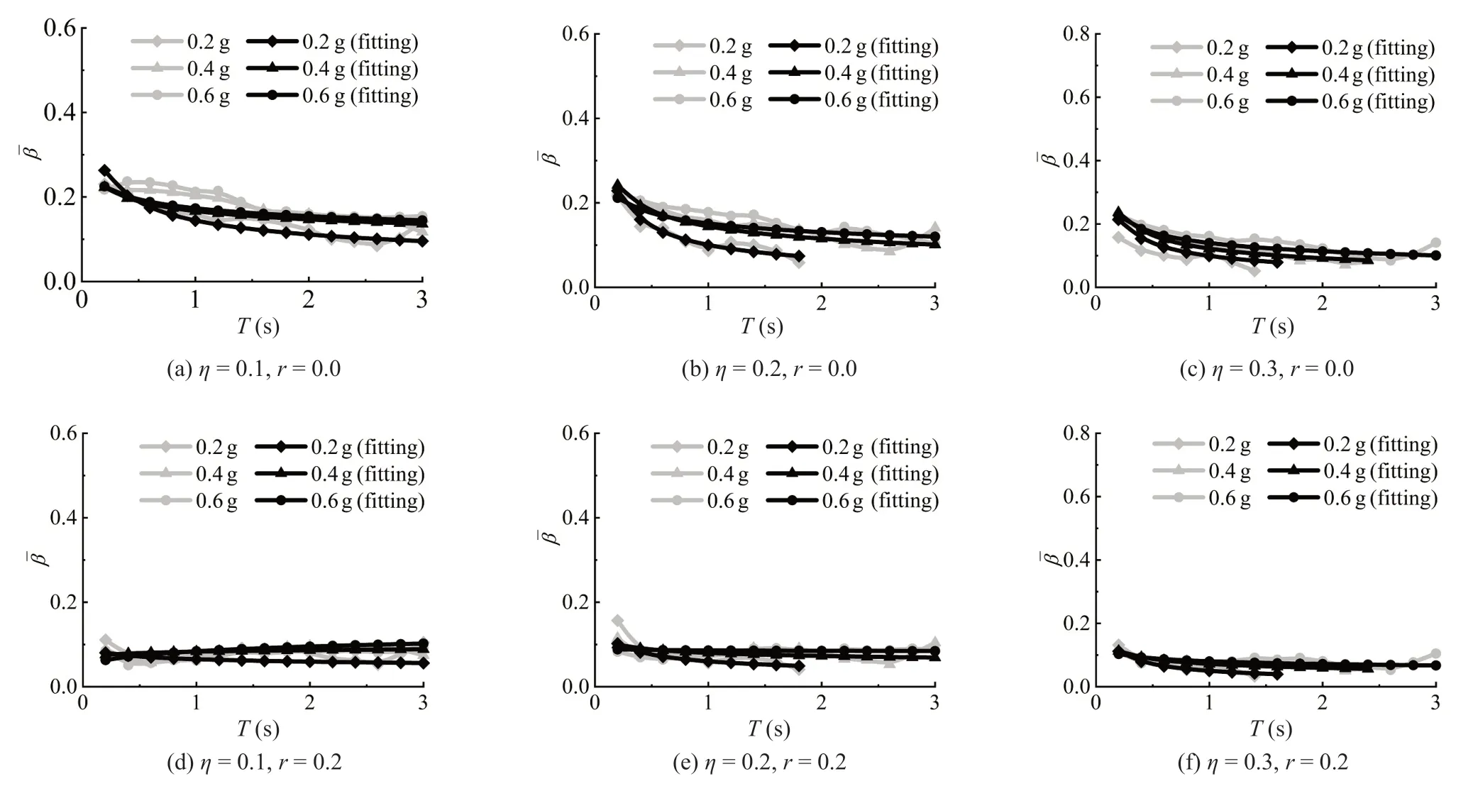
Fig. 6 Mean values of residual/maximum deformation ratio of SDOF systems based on T-model

To determine the mean values of the deformation ratio for the systems with different hysteretic behavior, Figs. 5 and 6 show the statistical results ofvs.Tfor the different bilinear SDOF systems, respectively, based on the K-model and T-model with a light line. As shown in Fig. 5, the mean deformation ratios () of the SDOF systems based on the K-model decrease as the period (T) increases, and the decreasing tendency is associated with parameters such as the stiffness ratio (r), relative yield force coefficient (η) and peak acceleration (apg) of the ground motion. Overall, the decreasing tendency ofvs.Tis relatively distinct in the short period region from 0 to 0.6 s and generally becomes stable in the long period region from 0.6 to 3 s. The mean values of the deformation ratio () decrease as the system stiffness ratio (r) and relative yield force coefficient (η) increases and increase as the peak ground acceleration (apg) increases. Note that the peak ground acceleration (apg) has little effect on the mean values of the deformation ratio () when the stiffness ratio (r) and the relative yield force coefficient (η) are large. Similarly, the mean value of the residual deformation ratios of SDOF systems based on the T-model tends to decrease as period (T) increases, as shown in Fig. 6. The dispersion of the mean values of the residual deformation ratio of SDOF systems based on the T-model is less than that based on the K-model because the hysteretic characteristics of stiffness degradation of the systems are considered with the T-model. Compared with the statistical results of the systems with the K-model, the relationship ofβvs.Tof the systems with the T-model is hardly affected by the peak ground acceleration, especially when the stiffness ratio and peak ground acceleration are large. Signifciantly, some data points of mean values () based on the K-model and T-model with long period regions (T) and large relative yield force coefficients (η) are not shown in Figs. 5 and 6, which is because the vast majority of 100 normalization seismic motion inputs with small seismic levels (e.g., PGA = 0.2 g) cannot enable these SDOF systems with given initial properties (e.g., large relative yield force coefficient) to enter the yielding stage; that is,pi< 10%, wherepiis the yielding ratio between the effective number (iN) and the total number (Nt= 100) of ground motion records. In other words, the SDOF systems in this situation can be assumed to not yield and remain in an elastic state, and the maximum seismic deformation is smaller than the corresponding yielding deformation. Therefore, the residual deformation prediction for SDOF systems in this situation may be unnecessary.

According to the tendency and influences of the stiffness ratio, relative yield force coefficient and peak ground acceleration on the−Trelationship for SDOF systems with different parameters, the mean values of the deformation ratio of the systems based on the T-model and K-model can be consistently expressed based on the optimized regression of the statistical results as follows:

where1Qand2Qare coefficients related to the stiffness ratio, relative yield force coefficient and peak ground acceleration, and can be determined according to the statistical results illustrated in Figs. 5 and 6.

For the K-model,1Qand2Qcan be estimated as follows:

For the T-model,1Qand2Qcan be estimated as follows:

The mean values of the deformation ratio of SDOF systems estimated by Eq. (3) are also shown in Figs. 5 and 6, which are described with the dark line. The results of the proposed Eq. (3) are found to correlate well with the statistical data points described with the light line mark.

To determine the coefficient of variation (βδ) of the deformation ratio for the systems with different hysteretic behaviors, Figs. 7 and 8 illustrate the statistical results of the coefficient of variation of the deformation ratio for the different bilinear SDOF systems based on the K-model and T-model with the light line, respectively. As shown in Fig. 8, a linear relationship between the coefficient of variation (βδ) and the period (T) of SDOF systems is observed for the K-model, which is related to the stiffness ratio (r) and relative yield force coefficient (η); that is, the linear proportionality coefficients for the relationship are influenced by the parametersrandηof the systems. However, note that the relationship betweenβδandTis barely affected by the peak ground acceleration (apg). This indicates that the uniform linear function can be used to describe the relationship ofβδ-Tof the systems subjected to different seismic excitation levels (i.e.,apg=0.2 g, 0.4 g and 0.6 g). Similar to Fig. 7, the linear relationship between the coefficient of variation (βδ) and the period (T) of SDOF systems based on the T-model is shown in Fig. 8. The linear relationship is significantly affected by the stiffness ratio (r) and relative yield force coefficient (η) but not by the peak ground acceleration (apg).

Fig. 7 Coefficient of variation (δβ) of deformation ratio of the systems based on K-model

Fig. 8 The coefficient of variation (δβ) of deformation ratio of the systems based on T-model

According to the influence trends of the stiffness ratio and relative yield force coefficient on the relationships ofβδ-Tfor SDOF systems with different parameters, the coefficient of variation (βδ) of the deformation ratio of the systems based on the T-model and K-model can be consistently expressed based on the optimized fitting of the statistical results as follows:

where1Q′ and2Q′ are coefficients related to the stiffness ratio and relative yield force coefficient and can be determined according to the statistical results illustrated in Figs. 7 and 8. For the K-model,1Q′ and2Q′ can be estimated as follows:

For the T-model,1Q′ and2Q′ can be estimated as follows:

The coefficients of variation (βδ) of the deformation ratios for SDOF systems were estimated by Eqs. (8)–(12) and are shown in Figs. 7 and 8, as described with the dark line. The predicted results correlate well with the statistical data points described with the light line. Certainly, it is noted that the residual deformation ratio (β) is not only affected by the peak ground acceleration (apg), period (T), stiffness ratio (r), relative yield force coefficient (η) and hysteresis characteristics, but also by the uncertainty and discreteness of the seismic response of the SDOF systems subjected to different seismic ground motions. Although the influences of all the parameters mentioned above on the residual deformation ratios are comprehensively considered, the empirical formulas (i.e., Eq. (3) and Eq. (8)) still have some unavoidable errors.

3.3 Probability distribution

To determine the probability distribution of the residual/maximum deformation ratio (β) of the SDOF systems, typical histograms and corresponding lognormal distribution fitting curves ofβfor the SDOF systems based on the K-model and T-model are illustrated in Fig. 9. From the figures, the probability distribution ofβapproximatively obeys a lognormal distribution, which is also consistent with the results of the Kolmogorov-Smirnov (K-S) test. The probability density function and distribution function ofβcan be written as follows:

Fig. 9 Histograms and probabilistic distributions of deformation response ratio of SDOF systems

µlnβandσlnβare the mean value and standard deviation of the deformation ratio (β) after taking the logarithm, respectively.andδβare the mean value and coefficient of variation ofβ, respectively, and can be estimated according to Eqs. (3) and (8). In Fig. 9,fβis the frequency of the samples ofβfalling into each interval of the histogram.

4 Establishment of an analytical model for the residual deformation of a SDOF system

The seismic deformation ratio (β) of SDOF systems can be assumed to be a random variable because of the uncertainty of ground motion records, and the possibility ofβexceeding a certain value (e.g.,dR/dm) can be expressed by the probabilityPβ. Sinceβobeys a lognormal distribution,Pβcan be written as the following expression:

whereΦ(⋅) is the standard normal distribution function.

Assuming that the probability (Pβ) is known, the seismic residual deformation of SDOF systems can be derived according to Eq. (17) as follows:

where ()1−⋅Φis the inverse of the standard normal distribution function. Note that the rationality of Eq. (17) is only based on the independent relationship between the residual deformation and the maximum deformation; the corresponding discussion on the correlation between the two deformations mentioned above have been made in previous studies (e.g., Kawashimaet al., 1998; Guo and Christopoulos, 2018) and it has been concluded that they can be regarded as independent of each other.

According to the proposed model (i.e., Eq. (17)), the maximum deformation (dm) should be known in advance to predict the seismic residual deformation (dR) of SDOF systems.dmcan be approximately predicted by the pushover method from a practical perspective. However, there are some differences between the pushover method and the nonlinear time history analysis method in predicting the maximum deformation of the systems due to the effects of record-to-record variability (Ruiz-Garcia and Miranda, 2006; Chenget al., 2013). The statistical relationships between the pushover method and the nonlinear time history analysis method in predicting the maximum deformations of SDOF systems have been established in the literature by Chenget al.(2013), and the probability-based model of the maximum possible deformations of SDOF systems subjected to seismic loading predicted by the pushover method is shown as follows:

wheredtmis the maximum deformation predicted by the nonlinear time history analysis method;dpmis the maximum deformation predicted by the pushover analysis method;Pαis the given exceeding probability;µlnαandσlnαare, respectively, the mean value and standard deviation of the maximum deformation ratioα(i.e., the ratio of the maximum deformations predicted by the nonlinear time history analysis and pushover analysis) after taking the logarithm; andandδαare the mean and coefficient of variation ofα. The detailed calculation formulas can be found in Chenget al.(2013).

5 Case study for residual deformation analysis and repairability evaluation of SDOF systems

To illustrate the method proposed herein for evaluating the residual deformation and repairability of SDOF systems, a case study of a seismic repairability assessment for a bridge structure with a single RC pier illustrated in Fig. 1 was conducted. The column pier is designed with the following properties: bridge heightHis 6000 mm; concentrated massmof the bridge structure is 3.8×105kg; cross-sectional dimensions are 1500 mm×1500 mm; twenty longitudinal reinforcing bars with a diameter of 32 mm, yielding strength of 360 MPa and ultimate strength of 500 MPa are distributed uniformly on four sides of the pier; transverse reinforcing bars with a diameter of 10 mm, yielding strength of 300 MPa and spacing of 100 mm are arranged in the pier. It was assumed that the bridge is located in a category Ⅲ site and corresponds to the second design seismic group according to the Chinese Seismic Design Code (GB 50011-2010, 2010). To illustrate the differences in seismic residual deformations of the bridge pier with different probability levels, the residual deformations with exceeding probabilities of 16%, 50% and 84% were evaluated by the model proposed in this study, and a preliminary analysis of the repairability of the bridge pier was carried out.

According to Eq. (17), the maximum nonlinear deformation (dpm) of the bridge pier should be estimated first by the pushover method. In the pushover procedure, the capacity curve (i.e., monotonic load-displacement curve) of the bridge can be obtained by sectional analysis technology and the plastic hinge method (Zhanget al., 2011). The nonlinear demand spectrum of the bridge based on the T-model and K-model is obtained from a 5% design spectrum, which is recommended by the Chinese Seismic Design Code (GB 50011-2010), reduced by the equivalent viscous damping considering the hysteretic energy dissipation. The equivalent viscous damping ratios (ζeq) for the T-model and K-model can be evaluated as follows:

The maximal displacement responses (dpm) of the bridge are 146.74 mm and 170.01 mm for the K-model and T-model, respectively, according to the capacity spectrum method, and the corresponding equivalent viscous damping ratios are 46.44% and 22.5%, as shown in Fig. 10. In this figure, pointYis the pier column yield point, which corresponds to the first yielding of the reinforcing bars in tension.

Fig. 10 Seismic performance points of bridge pier

Assuming that the exceeding probability (Pα) is 50%, the maximum deformation (dtm) and the maximum drift ratio (mθ) of the top of the bridge pier can be obtained for the K-model and T-model by Eq. (17), and the predicted results are listed in Table 1. It can be seen from the table that the maximum drift ratio (mθ) for the K-model and T-model are all less than the threshold limit value (i.e., [mθ] = 1/30) recommended in the Chinese Seismic Design Code (GB 50011-2010). This suggests that the designed bridge pier meets the maximum nonlinear deformation requirements under a given seismic intensity level and that the residual deformation and repairability of a bridge should be considered in terms of a nonfatal collapse.

According to the analytical results mentioned above, the related parameters of the bridge pier for the K-model and T-model can be conveniently determined, such as the natural period (T), relative yield force coefficient (η), stiffness ratio (r) and ground peak acceleration (apg). Then, combining Eqs. (3), (8), (13) and (14), the mean value (lnβµ) and standard deviation (lnβσ) of the logarithm of the residual deformation ratio (β) can be obtained. Additionally, the seismic residual deformation (dR) and the corresponding residual deformation drift ratio (θR) of the bridge pier with exceeding probabilities (Pβ) of 16%, 50% and 84% can be obtained according to Eq. (17), as listed in Table 2.

Table 1 Predicted results of the dtm and θm of the bridge

Table 2 Predicted results of related parameters of the bridge

From Table 2, it can be seen that the residual deformation drift ratios (Rθ) based on the K-model and T-model are all less than the threshold limit value (i.e., [θR] = 1.75%), which is recommended by the Design Specifications of Highway Bridge (Part V: Seismic Design) (2002) of Japan. This indicates that the reparability capacity of the designed bridge in the case study is well under the given probability levels. Note that the predicted seismic residual deformation decreases and the corresponding repairability probability of the bridge under the given seismic excitation increases with the increase in the given exceeding probability. Furthermore, the analytical results based on the K-model with nondegrading hysteretic behavior are larger than those based on the T-model with degrading hysteretic behavior; that is, the analytical results of the repairability for the structures with the K-model are more conservative.

To further illustrate the reasonability of the proposed model, the K-model based residual deformation model (i.e., Eq. (17) with K-model) is compared with the method of residual deformation spectrumRcpresented by Kawashima and MacRaeet al. (1998). Their model was established based on the bilinear hysteretic model with non-degrading hysteretic behaviors (i.e., K-model), and was also adopted by the Design Specifications of Highway Bridge (Part V: Seismic Design) (2002) of Japan. The equation of the model is as follow:

wherecRis defined as the ratio of residual deformation to theoretical maximum residual deformation, which is mainly related to the stiffness ratio (r) and can be determined by the residual deformation response spectrum suggested by the Japanese code; andµ∆is the displacement ductility coefficient. Substituting the relative parameters (i.e.,r,dy,dtmandcR) of the bridge structure described in the case study into Eq. (23), the predicted residual deformationdRis 49.75 mm. This result is approximately equal to the predicted result of Eq. (17) based on the K-model when the given transcendence probabilityP(β) is 16%, as listed in Table 2. This means that the prediction of residual deformation of SDOF systems by using the proposed model (i.e., Eq. (17)) has a high reliability. However, note that the residual displacement spectrumcRgiven in the Japanese code is primarily determined based on the mean values of the nonlinear time history analysis results which ignore the effects of dispersion and uncertainty of the results. Therefore, the upper and lower limits of the residual displacement spectrumcRwith plus or minus one time standard deviation from the mean values were also suggested in the Japanese code to consider the prediction dispersion. In this case, the range of residual displacement prediction of the bridge described in the case study is 12.44 mm – 96.74 mm according to the Japanese code. The wide margins of the results indicate that the residual displacements of the structures should be predicted considering the effect of dispersion, and the residual displacement model proposed from the viewpoint of probability may be more reasonable and suitable, which is more consistent with the performed-based design philosophy. In addition, a simplified residual deformation model was also provided in the Seismic Performance Assessment of Buildings (FEMA P58, 2012), and the residual deformations of the systems depend on the repairable probability, maximum displacement and yielding displacement. According to the model suggested in FEMA P58, the residual deformation (dR) of the system is equal to the maximum deformation (dm) minus three times the yielding displacement (3dy) when the displacement ductility coefficient is larger than 4.0. Hence, the residual deformation of the bridge described in the case study is 69.14 mm, which is a deterministic value and is approximately equal to the predicted result of Eq. (17) based on the K-model when the given transcendence probability ()Pβis 6%. This comparison also suggests that the proposed model (i.e., Eq. (17)) is more reasonable and robust, and is more suitable for simplified performance assessment and design for considering the seismic repairability.

Table A1 Continued

Table A1 Continued

Table A1 Continued

Table A1 Characteristics of recorded earthquake ground motions

6 Conclusions

The elastoplastic seismic responses of different SDOF systems based on kinematic/Takeda hysteretic models under a series of normalized ground motion records were statistically analyzed, and the effects of the uncertainty of the model parameters and seismic records on the residual deformation of SDOF systems were studied. The conclusions are as follows.

(1) There is obvious dispersion of the analytical results of the ratios of seismic residual deformation to maximum deformation (dR/dm) of SDOF systems under different seismic ground motion records. The dispersion degree of the residual deformation ratio (dR/dm) is mainly influenced by the stiffness ratio, hysteretic model, natural vibration period, relative yield load coefficient and peak ground acceleration.

(2) The statistical distribution of the residual deformation ratio (dR/dm) of SDOF systems based on the bilinearK/Thysteretic models can be described by the lognormal distribution function. A power function and linear function can be adopted for characterizing the relationship between the mean value and the structural period (T) and that between the coefficient of variation andT, respectively.

(3) The proposed model based on a lognormal distribution function can be used to predict the residual deformations of SDOF systems under the given probability requirements and seismic levels. The analytical results of residual deformation based on the K-model is more conservative than those based on the T-model.

(4) The proposed probabilistic model of residual deformation of SDOF systems in this study is focused on the known maximum deformation, which can be estimated by the pushover method or other methods reported in the literature. Additionally, the proposed procedure can predict the residual deformation when the displacement ductility demand of a SDOF system is unknown.

Acknowledgment

This study was funded by the Natural Science Foundations of China (Grant Nos. 51508154, 51978125 and 51678104), the Natural Science Foundation of Jiangsu Province (BK20211206), the Fundamental Research Funds for the Central Universities (B210202033), China Postdoctoral Science Foundation (2020M670787), and the Priority Academic Program Development of Jiangsu Higher Education Institutions. The authors wish to express their gratitude for this support.

Appendix