Geotechnical engineering blasting: a new modal aliasing cancellation methodology of vibration signal de-noising

Yi Wenhua, Yan Lei, Wang Zhenhuan, Yang Jianhua, Tao Tiejun and Liu Liansheng

1. School of Resource and Environmental Engineering, Jiangxi University of Science and Technology, Ganzhou 341000, China

2. School of Civil Engineering and Architecture, Nanchang University, Nanchang 330031, China

3. School of Civil Engineering, Guizhou University, Guiyang 550025, China

Abstract: In the present study of peak particle velocity (PPV) and frequency, an improved algorithm (principal empirical mode decomposition, PEMD) based on principal component analysis (PCA) and empirical mode decomposition (EMD) is proposed, with the goal of addressing poor filtering de-noising effects caused by the occurrences of modal aliasing phenomena in EMD blasting vibration signal decomposition processes. Test results showed that frequency of intrinsic mode function (IMF) components decomposed by PEMD gradually decreases and that the main frequency is unique, which eliminates the phenomenon of modal aliasing. In the simulation experiment, the signal-to-noise (SNR) and root mean square errors (RMSE) ratio of the signal de-noised by PEMD are the largest when compared to EMD and ensemble empirical mode decomposition (EEMD). The main frequency of the de-noising signal through PEMD is 75 Hz, which is closest to the frequency of the noiseless simulation signal. In geotechnical engineering blasting experiments, compared to EMD and EEMD, the signal de-noised by PEMD has the lowest level of distortion, and the frequency band is distributed in a range of 0–64 Hz, which is closest to the frequency band of the blasting vibration signal. In addition, the proportion of noise energy was the lowest, at 1.8%.

Keywords: blasting vibration; frequency; empirical mode decomposition; modal aliasing; de-noising

1 Introduction

During on-site blasting vibration (Blair, 2015; Yanet al., 2017) test processes, due to the interference of external factors, as well as factors related to the vibration meters themselves, random noise often exists in vibration signals (Parket al., 2009). This noise will potentially affect the analysis results of the vibration signals. Therefore, PPV (Lianget al., 2013) and frequency (Cohen, 1994; Lianget al., 2013; Zhouet al., 2016) analyses of the signals is required in order to remove the influence of noise. At present, the most commonly used signal de-noising methods include Fourier transform, wavelet transform, Hilbert-Huang transform (HHT), and so on. Among these methods, the Fourier transform denoising method (Zhai, 2014; Mateo and Talavera, 2018; Wang and Liu, 2019) had become the most traditional method used to address unwanted signal noise. Generally, Fourier transform is first carried out on the signals, followed by inverse transform after a filtering process has been completed. However, since Fourier transform can only be analyzed in the frequency domain, if a signal suddenly changes somewhere in the time domain, it will affect the entire frequency domain. In such cases, it becomes impossible to distinguish whether the spike of the signal has been caused by sudden change or by noise. To address this issue, a wavelet transform theory (Ercelebi, 2014; Cuiet al., 2016; Bayeret al., 2019) was introduced in the 1980s. The wavelet transform theory can transform signals in the time and frequency domains. For example, for analysis, a wide time window can be used for low frequency components of signals, while a narrow time window can be used for high frequency components. In this way, better de-noising effects can be achieved. However, the accuracy of wavelet transform decomposition is dependent on the selection of the wavelet basis. This selection has a certain fuzziness and its length is limited, which may result in signal energy leakage. Therefore, it has become necessary to determine a more effective time-frequency analysis method to solve this leakage problem. It has been found that the HHT transform (Hanet al., 2014; Dinget al., 2007; Penget al., 2012), which is composed of the Hilbert transform and empirical mode decomposition (EMD) (Huanget al., 1998; Nagarajaiah and Basu, 2009; Tianet al., 2015; Shiet al., 2016) can directly decompose original signals into a series of intrinsic mode function (IMF) components, from high- to low-frequency levels according to different time scales. This can be used to accurately extract the characteristics of nonstationary signal changes. When compared with wavelet transform methods, it has been observed that the HHT does not require the selection of a basis function and is characterized by self-adaptability and multi-resolution. Furthermore, the HHT can perform more effective time-frequency analyses of non-stationary signals. However, during actual filtering and de-noising processes, it has been found that the HHT may also encounter some problems, such as the occurrence of modal aliasing phenomena (Wu and Huang, 2009; Huet al., 2012; Damaseviciuset al., 2017) between IMF components decomposed by EMD. For example, the decomposed IMF components will be unable to meet the sequential digression of the frequencies and uniqueness of the dominant frequency, which will potentially affect the de-noising effects of HHT filtering processes.

At present, with the goal of addressing the problem of IMF component aliasing, Momeniet al. (2018) proposed an auxiliary function consisting of highfrequency components and low-frequency components, which corresponded to the noise and dominant frequencies added to the data, for the purpose of enhancing each of the IMF components and avoiding overlapping among the components. Damaseviciuset al. (2017) proposed a scale adaptive remixing de-noising method of intrinsic mode functions (IMFs) based on EMD. The results revealed that the method had solved the incomplete decomposition problem by adopting a heuristic algorithm with the least correlation between the first-order modulus and the generated second-order modulus subset. Huet al. (2012) presented a new definition for the envelope of the IMF components and introduced an envelope approximation algorithm. Wu and Huang (2009) proposed ensemble empirical mode decomposition (EEMD) (Liet al., 2016) for the suppression of the incomplete orthogonality between the IMF components. It was determined that the EEMD method required advance calculations of signal-to-noise ratios, which resulted in poor suppression effects for mixed signals with low frequency ratios.

Although the above-mentioned methods all have their own advantages in solving modal aliasing problems, they all have displayed certain limitations. In the present study, principal component analysis (PCA) (Hotelling, 1936; Wiseet al., 1990; Spiegelberg and Rusz, 2017; Fuentes-Garcíaet al., 2018) was introduced to address these short-comings. In this study, PCA was used to improve the EMD, and a principal empirical mode decomposition (PEMD) filtering de-noising method was proposed. The IMF principal component sets decomposed by EMD were converted into a small number of orthogonal IMF principal component sets to remove modal aliasing effects. As a result, the filtering and de-noising processes could more effectively be performed.

2 Improved algorithm

2.1 PCA principle

The PCA is the projection of a high-dimensional vectorXinto a low-dimensional vector space through a special eigenvector matrixU, expressed by a lowdimensional vectorY, with only the loss of a small part of information or secondary information. For example, a group of two-dimensional random arraysis displayed on a two-dimensional plane, as shown in Fig. 1.

Fig. 1 Data point distribution diagram

To reduce the array dimension and improve the analysis result, according to the maximum variance theory (Shao and Rong, 2009; Liuet al., 2014; Weiet al., 2016) the maximum variance direction of the twodimensional random arrays is theX-axis direction. Therefore, it is projected onto theX-axis, and the projection point is taken as a new one-dimensional random array, as shown in Fig. 2.

Next, a new low-dimensional orthogonal array can be obtained, which has inherited the majority of the eigenvalues of the original array, independently of one another.

When the maximum variance direction of a twodimensional random array will not be in the direction of the coordinate axis (X-axis andY-axis), it is displayed on a two-dimensional plane, as shown in Fig. 3.

Fig. 2 Orthogonal projection of the random number point

Fig. 3 Orthogonal projection of the new coordinate axis and the maximum direction of the variance

Meanwhile, the maximum direction of the variance will be a straight line with a slope of 1 (i.e., the optimal projection axis). The assigned distance between the projection point and the origin point will be taken as the substitute value of the original data point. In this way, a group of two-dimensional arrays can be successfully converted into a one-dimensional orthogonal array on the new coordinate axis, using PCA. Therefore, PCA can transform a large number of correlated high-dimensional arrays into a set of orthogonal, low-dimensional feature components.

2.2 Details of the improved algorithm

An improved algorithm PEMD was proposed in this study for the purpose of solving a problem, namely, that an incomplete orthogonal decomposition of the EMD negatively affected filtering and de-noising processes. First, the original signal was decomposed by the EMD to obtain a series of IMF components. Next, the decomposed IMF components and the original signal were subjected to a principal component analysis process to obtain the orthogonal multiple principal components. In the present study, in accordance with the contribution rates of each of the principal components, the principal components containing the majority of the information from the original signal were selected to be combined into an orthogonal, original signal reconstruction. At that point, the orthogonal IMF components could be successfully decomposed by EMD orthogonal decomposition. The specific algorithm steps were taken as follows:

Step 1: Extraction of the original data

The original signal ()xtwas decomposed intomIMF components using EMD, and thensample points were obtained for each of the components.

Step 2: Standardization of the original data

It was assumed that the IMFs for principal component analysis and the value of thej-th IMF component of thei-th sample point was taken asaij, which was then converted into a standardized value.

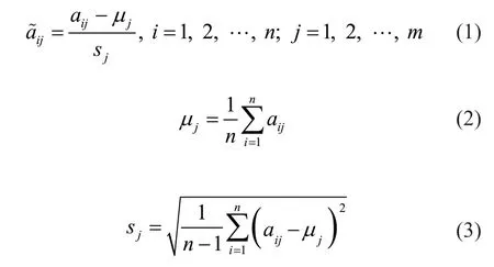
In the equation,μjis the mean of thej-th IMF component; andsjis the standard deviation of thej-th IMF component.

Meanwhile, the IMF components were standardized.

In the equation,jx~ represents the standardized IMF components.

Step 3: Calculation of the correlation coefficient matrixR

Step 4: Calculations of the eigenvalueλjand the eigenvectorμj

The eigenvalueλjof the correlation coefficient matrix is calculated and the corresponding eigenvectormis obtained.

Step 5: Calculation of the cumulative contribution rate

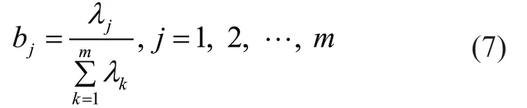
In the above equation,bjis the information contribution rate of the principal component, andαprepresents the cumulative contribution rate of the firstpprincipal components.

Step 6: Selection of the IMF principal component combination

Select principal components with a cumulative contribution rateαpof 90% (Maćkiewicz and Ratajczak, 1993) or more. Since the principal components are completely orthogonal, orthogonal original signalsx′(t) can be constructed, with a contribution rate of each principal component as the weight.

Step 7: EMD

EMD is performed on the orthogonal original signalx′(t) to obtain a fully orthogonal IMF component.

This study′s algorithm flow chart is shown in Fig. 4.

Fig. 4 PEMD algorithm flow chart

Fig. 5 The original analog signal

3 Simulation experiment

This study had selected the cosine signalx1(t)=2cos(150πt) as an example. Since the probability density function of Gaussian white noise (Elad and Aharon, 2006; Biet al., 2015) had satisfied the statistical characteristics of a normal distribution—which can truly reflect the noise characteristics of vibration signals—it was found that the function could be accurately represented by a specific mathematical expression. Therefore, the original analog signal in the present study consists of a cosine signal and a Gaussian white noise signal with a one-dimensional probability density ()pt, denoted as()xt.

The sampling frequency was set as 1,024 Hz, the number of sampling points was 100, and the signal length was 0.1 s. The original analog signal waveform, mixed with Gaussian white noise, is shown in Fig. 5.

It can be seen in Fig. 5 that the original analog signal was formed by the superposition of a cosine signal, with an amplitude of 2 and a frequency of 75 Hz, plus Gaussian white noise with an average value of 0 and a variance of 0.9. The original analog signal was decomposed by EMD for the first time to obtain a series of IMF components (Chenget al., 2006) from high- and lowfrequency ranges. Then, each component was subjected to a Fourier transform to obtain its own frequency spectrum, as shown in Fig. 6.

From the IMF component on the left part of Fig. 6, it is clear that IMF1 denotes the Gaussian noise signal, and IMF2 and IMF3 indicate the decomposed cosine signals. However, due to noise interference, there were no obvious cosine characteristics observed, which resulted in aliasing phenomena. Also, IMF4 and IMF5 represent the components with lower frequencies, following the decomposition process, and IMF5 indicates the drift of the measuring instruments or the trend term of the signals.

The results from the additional analysis of the spectrum (on the right part of Fig. 6) had indicated that the frequency distribution of the IMF1 Gaussian noise had ranged between 0 and 500 Hz, and that of the IMF2 had also been distributed in the range of 0 to 500 Hz. Meanwhile, it was observed that the IMF2 had displayed a variety of dominant frequencies that were not unique. The frequency band of IMF3 had ranged between 0 and 200 Hz, with two main frequencies observed. The frequency band of IMF4 ranged between 0 and 150 Hz, and it was found that IMF4 had multiple dominant frequencies. The frequency distribution of IMF5 was in the range of 0 to 100 Hz, which had not conformed to the law of decreasing in sequence. The same was observed for the frequency distribution range of IMF6 (0 to 200 Hz). Therefore, it was determined that each of the IMF decomposed components had not conformed to the law of frequency oneness and decreasing in sequence in the EMD, which had resulted in the occurrences of aliasing phenomena. Therefore, the first EMD of the original signal had directly led to serious aliasing phenomena, and all the IMF decomposed components had experienced noise interference. Subsequently, filtering and de-noising processes could not be effectively carried out.

In the present study, for the purpose of effectively removing noise interference from the EMD, the abovementioned signals were analyzed using a PEMD improvement algorithm. First, the original signal was EMD decomposed, and a total of six IMF components were obtained. Then, the IMF component map and the original signal were utilized to derive the total data for principal component analysis. Next, the eigenvalues and the eigenvectors of the correlation coefficient matrix of IMF components were calculated, as shown in Table 1.

Table 1 The eigenvectors and the eigenvectors of the correlation coefficient matrix

And the cumulative contribution rates of the eigenvaluesλjare shown in Fig. 7.

As can be seen in Fig. 7, the cumulative contribution rates of the first five eigenvalues had reached 90% of the original information. It is assumed that the first five new principal components, composed of the first five eigenvectors, contain most of the original signal information. Then, since the principal component analysis could effectively transform the original variables into completely orthogonal variables, the five variables were found to have orthogonality with one another. Therefore, the first five new variables were selected as the principal components in the reconstruction of the signal, and then EMD was carried out for the purpose of obtaining completely orthogonal IMF components. A comparison was then made between the IMF components obtained by EMD and those obtained using EEMD, as shown in Fig. 8.

Fig. 6 The six IMF components of EMD and corresponding spectrum diagram

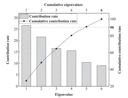
Fig. 7 The contribution rates of the eigenvalues

As can be seen in Fig. 8, IMF1 represents the Gaussian noise signal, and IMF2 indicates the decomposed cosine signal. It was clear that the PEMD had obvious cosine characteristics when comparing the IMF2 decomposed by the EMD and EEMD methods. Therefore, it was determined that the degree of noise interference had been reduced. The results of this study′s further analysis of the improved spectrum are shown in Fig. 9.

As shown in Fig. 9, the IMF1 decomposed by the EEMD and EMD methods were Gaussian noise, with a frequency distribution range of 0 to 500 Hz. The frequency range of IMF2 was between 0 and 500 Hz, with various dominant frequencies observed. The frequency range of the IMF3 obtained by EEMD was between 0 and 200 Hz. It was found that when compared with IMF components obtained by EMD, although the dominant frequency was not unique, the aliasing phenomena tended to be weakened. However, the spectrum distribution range of the IMF4 decomposed by EEMD had ranged from 0 to 500 Hz. When compared with the IMF3, it was found to be inconsistent with the law of decomposition frequency decreasing in sequence and was similar to frequency distribution ranges of IMF6 and IMF5. Therefore, it was found in this study that compared with the EMD, the EEMD method had reduced the aliasing phenomena to some extent.

Fig. 8 IMF component comparison chart prior to and after improvements

However, the frequency bands of each of the IMF components obtained by PEMD had been in the ranges of 0 to 500 Hz, 0 to 400 Hz, 0 to 300 Hz, 0 to 200 Hz, 0 to 150 Hz, and 0 to 100 Hz in sequence, respectively. The frequency distribution ranges were observed to be in a state of decreasing in sequence, and the dominant frequency of each component was found to be unique. Therefore, each component of PEMD had displayed both decreasing frequency and uniqueness of dominant frequency following the decomposition, which had obviously eliminated the aliasing phenomena and enabled improved filtering and de-noising processes. In the present study, signals had been filtered using EMD, EEMD, and PEMD, respectively. It was determined that since the signal components were relatively single, fewer IMF components had been obtained by EMD, EEMD, and PEMD. As a result, the filtered and denoised signals were mainly concentrated in the IMF2 component. Therefore, the principal component, IMF2, was selected for purposes of analysis, and respective frequency spectra were created in order to compare the de-noised effects of the three components, as illustrated in Fig. 10.

As can be extrapolated from the analysis results displayed in Fig. 10(a), the filtering and de-noising effects of the PEMD were superior to those of the EEMD and EMD. Further analysis revealed that the evaluation rules (Zhonget al., 2014) were based on the signalto-noise ratios (SNR) (Chen and Yu, 2007; Gonzalez-Morenoet al., 2014; Gómez-Chovaet al., 2018), and root mean square errors (RMSE) had been adopted. The higher the SNR and smaller the RMSE, the better the denoising effect would be, i.e., the higher the ratio of SNR and RMSE, in turn the better the de-noising effect would be. To synthesize these two evaluation indexes, the ratio of SNR and RMSE is taken to evaluate the de-noising effect of different methods. The de-noising effects of the three methods were subsequently evaluated, as shown in Table 2.

As can be seen in Table 2, the SNR/RMES values were as follows: PEMD > EEMD > EMD. Therefore, the de-noising effects of the PEMD had been determined to be superior to those of the EEMD and EMD in the present study.

Table 2 Evaluation index of the de-noising effects in the analog signal

As shown in the spectrum analysis results presented in Fig. 10(b), the dominant frequency of the pure analog signal was 75 Hz and the amplitude of dominant frequency was 100. The main frequencyafter EMD filtering and de-noising had been distributed in the range of 55 to 110 Hz and had obviously contained noise interference. Additionally, the amplitude of the dominant frequency had not reached 100. The dominant frequency of the EEMD filtering and de-noising was determined to be 75 Hz. However, the amplitude of the dominant frequency did not reach 100. As a result, part of the vibration signal energy had been lost. In contrast, it was determined that the main frequency after PEMD filtering and de-noising had been 75 Hz and the amplitude of dominant frequency had reached 100, with no loss of energy observed. Therefore, as viewed from the comparison results of the frequency ranges and energy, the PEMD had displayed the best filtering and de-noising effects.

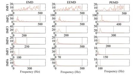
Fig. 9 Spectrum comparison chart prior to and after improvements

Fig. 10 Comparison of filtering and de-noising effects

Fig. 11 Blasting vibration signals and reconstructed signals

4 The blasting vibration signal

A group of data obtained from related literature (Zhanget al., 2019) was selected for analysis. The reconstructed orthogonal signal diagram through PEMD is shown in Fig. 11.

As shown in Fig. 11, the root mean square error (RMSE) of the reconstructed orthogonal signal and the original signal is 0.33%, so there is no distortion.

Therefore, the group of data was selected for EMD, EEMD, and PEMD filtering and de-noising processes. Because the blasting vibration signal contains a variety of complex noise components, and there is no blasting vibration signal with absolutely no noise, the SNR cannot be used to effectively evaluate the de-noising effects of the different methods. However, the noise will cause distortion in the blasting vibration signal (Yaoet al., 2015) and will exert a significant influence on the frequency and energy of the blasting vibration signal. Thus, the de-noising effect of different methods can be comprehensively evaluated from these three aspects. Additionally, the respective waveform and spectrum following de-noising are shown in Fig. 12.

As can be seen from the time domain signal shown in the left section of Fig. 12, the blasting vibration signals were contaminated by noise, the EMD and EEMD filtering de-noising methods were able to filter out part of the noise. However, when compared with the results obtained using the PEMD method, the de-noised signal still contained a large noise component. It was observed that the signal obtained by use of the PEMD filtering de-noising method was smoother, and more noise interference had been removed. As a result, the PEMD method had been found to be the most effective in the de-noising of the signal. Also, in accordance with the spectrum analysis shown in the right-hand section of Fig. 12, the dominant frequency band of the blasting vibration signal had been distributed within the range of 0 to 130 Hz. It was found in this study that according to the relevant literature (Zhanget al., 2019), the dominant frequency band of the blasting vibration signals of the Yongping Copper Mine was distributed in the range of 0 to 64 Hz. Therefore, it was confirmed that the blasting vibration signals were polluted by high-frequency noise. The dominant frequencies of the signals which had been de-noised by the EMD and EEMD filtering methods were distributed in the range of 0 to 95 Hz, which indicated that some of the high-frequency noise had been suppressed. However, the dominant frequency of the PEMD filtered and de-noised signal had been distributed in the range of 0 to 64 Hz, which indicated that most of the high-frequency noise had been filtered out. Therefore, the filtering effects of the PEMD were confirmed to be superior to those achieved using the EEMD and EMD methods in the time and frequency domains.

The stacked columnar energy diagram is shown in Fig. 13.

Fig. 12 Comparison of the de-noising effects

Fig. 13 Energy distribution of each frequency band and the energy percentage of the noise

It can be seen that the energy of the blasting vibration signals had decreased from a low to a high frequency, and then had increased once again. This was because the original signal had contained low-frequency vibration signals and more high-frequency noise. Meanwhile, the energy of the signals filtered by the EMD, EEMD, and PEMD methods had decreased from a low to a high frequency. Since the three examined methods had all filtered out some of the high-frequency noise energy, the signal energy of the medium and low frequencies had remained.

As shown in the vibration signal-noise broken line energy proportion diagram in Fig. 13, the vibration signal energy percentages of the EMD, EEMD, and PEMD had gradually increased, and the noise energy proportion had gradually decreased. Therefore, following the filtering, the three methods had successfully achieved de-noising effects. However, the vibration signal energy proportion of the PEMD method had reached more than 98.2%. It was observed that the noise had then only accounted for approximately 1.8%, which indicated that the majority of the noise energy had been effectively removed. Therefore, from the perspective of energy, the results obtained in this study verified that the PEMD method had displayed the best de-noising effects.

5 Discussion

During this study′s experimental process, it was found that a number of IMF components from the EMD of the same signal were unstable. It was observed that each IMF screening process had affected the validity and accuracy of the decomposition results, which had naturally impacted the subsequent filtering effects. Therefore, it was believed that if the screening was incomplete, the IMF components would be unable to fully express all the characteristics of the original signal. Additionally, if the number of screening layers was too large, then only some constants could be obtained, which would provide no practical physical significance. To address these issues, Huanget al. (1998) created a screening evaluation basis. For example, the standard deviation coefficient SD was utilized as the EMD component termination standard, to ensure that the screening times had a certain reference basis. However, it was found that only when the SD value was appropriate could a stable decomposition effect be achieved. Therefore, the criterion still possessed unstable convergence characteristics. Subsequently, Huanget al. (2001) had proposed two screening termination conditions through in-depth research of the EMD process and combining the conditions with an upper bound envelope. The results indicated that the decomposed IMFs had better mean value characteristics. However, the above-mentioned research methods were all based on technical improvements on the limitations of the EMD algorithm. Therefore, to obtain a relatively stable decomposition effect, this study proposed a PEMD method based on the characteristics of the original signal itself. It was believed that the instability of the EMD was ostensibly due to the setting of the screening termination conditions. However, it was revealed from actual results that the original signal had inherently not been completely orthogonally decomposed during the screening process. Meanwhile, different signals, to a certain extent, randomly decomposed into IMF components, which in each case led to instability in the decomposition results. As a result, various phenomena had occurred, such as modal aliasing. In the present study, based on inheriting the EMD adaptive decomposition of signals, the PEMD method was used to decompose the original signals strictly in accordance with the principle of complete orthogonality. The sub-signals with different characteristics were separated individually to ensure that the results obtained from each decomposition were completely consistent. It was found that when compared with the method of passive parameter selection, which is dependent on the decomposition effects being in line with the screening criterion, the PEMD had displayed major initiative and universality, thereby effectively solving the instability problem of the EMD.

Although the PEMD method was able to solve the problems of instability and incompleteness in the decomposition processes, and the filtering denoising effects were found to be better than those of EMD and EEMD, it was understood that the PEMD method still had its own limitations. Those limitations were dependent on the theoretical basis of principal component analysis. During the process of selecting the principal components, approximately 5% of the original information may be lost, which would make it unsuitable for the analysis of precision signals.

6 Conclusions

In this study, to solve the modal aliasing problem of vibration signal de-noising, a series of de-noising tests were designed and performed by observing the examples of simulation signals and the vibration signals of geotechnical engineering blasting. The following conclusions were drawn:

(1) EMD was successfully improved based on a principal component analysis method, and an improved algorithm PEMD for eliminating modal aliasing was proposed.

(2) In the simulation experiment, the SNR and the RMSE ratio of the signal de-noised by PEMD was the largest, compared to EMD and EEMD. The higher the SNR and smaller the RMSE, the better the de-noising effect. Thus, PEMD demonstrated the best de-noising effect. In addition, the main frequency of the de-noising signal through PEMD was 75 Hz, which was closest to the frequency of the noiseless simulation signal, and there was no energy loss after de-noising.

(3) In the geotechnical engineering blasting experiments performed in this study, compared with EMD and EEMD, the signal de-noised by PEMD had the lowest distortion degree; the main frequency of signal denoising by PEMD was in the range of 0–64 Hz, which was closest to the blasting vibration signal frequency range of the Yongping Copper Mine; and PEMD registered the lowest proportion of noise energy, only about 1.8%, thereby effectively filtering out most of the noise.

Acknowledgement

This work is supported by the National Natural Science Foundation of China (52064015, 51404111), the Jiangxi Provincial Natural Science Foundation (20192BAB206017), the Scientific Research Project of the Jiangxi Provincial Education Department (GJJ160643), the Program of Qingjiang Excellent Young Talents, and Jiangxi University of Science and Technology (JXUSTQJYX2016007). The authors wish to express their thanks to all of these supporting institutions. Additionally, special thanks go to the editor and the reviewers of this study, and for all their useful comments, which substantially improved the manuscript.