Response prediction using the PC-NARX model for SDOF systems with degradation and parametric uncertainties

Gao Xiaoshu, Chen Cheng, Hou Hetao and Jiao Shenghu

1. School of Civil Engineering, Shandong University, Jinan 250100, China

2. School of Engineering, San Francisco State University, San Francisco 94132-1722, USA

3. Shandong Engineering & Technology Research Center for Green Building and Intelligent Construction, Jinan 250100, China

Abstract: Building collapses during recent earthquakes have brought up the need for research on factors pertaining to collapse and the safety of structures. This requires response replication of structures that account for uncertainties from ground motions and structural properties. Structural collapse often implies that the structural system is no longer capable of maintaining its gravity load-carrying capacity, which often points to factors involving strength and stiffness degradation. In this study, the polynomial chaos nonlinear autoregressive with exogenous input form (PC-NARX) model is explored for dynamic response replication of a nonlinear single-degree-of-freedom (SDOF) structure. The generalized hysteretic Bouc-Wen model is applied to emulate stiffness and strength degradation for an SDOF structure close to collapse. A stochastic ground motion model is used to represent the uncertainties in seismic excitation. The PC-NARX model is employed and further evaluated for response replication of an SDOF system with inherent uncertain structural properties. A generic algorithm (GA) is used to select the terms for structural dynamics, and polynomial chaos expansion (PCE) is used to incorporate uncertain parameters into NARX model coefficients. It is demonstrated that the PC-NARX model provides good accuracy to account for both ground motion and structural uncertainties into response replication of SDOF structures with significant strength and stiffness degradation. The PC-NARX model thus presents a promising technique for collapse safety analysis of structures.

Keywords: polynomial chaos expansion; NARX model; hysteresis; degradation; collapse

1 Introduction

In recent years, there has been increasing interest in nonlinear behavior related to hysteresis in structural systems (Spaconeet al., 1996; Triantafyllouet al., 2012). The term hysteresis often refers to the main nonlinear phenomenon of structural behavior under the influence of earthquakes, which is usually accompanied by stiffness and strength degradation (Talatahariet al., 2012). With regard to engineering and structural fields, conventional buildings or structures may experience highly nonlinear hysteretic behavior for energy dissipation when subjected to natural hazards such as earthquakes. It is therefore important for engineers to incorporate nonlinear hysteretic behavior into response prediction for structures. Performance-based earthquake engineering (PBEE) also necessitates the development of reliable nonlinear analysis models that can replicate structural behavior under the influence of earthquakes (Lignos and Krawinkler, 2011). Building collapses during recent earthquakes have raised questions about how to determine the collapse safety margin of structures, what is the inherent collapse safety margin in codedesigned structures, and how to strengthen structures to effectively augment such a margin (Villaverde and Roberto, 2007). In earthquake engineering, collapse implies that the structural system is no longer capable of maintaining its gravity load-carrying capacity in the presence of seismic effects, which makes it necessary to simulate structural response far into the inelastic range, in which components deteriorate in strength and stiffness (Vamvatsikos and Cornell, 2006; Krawinkler and Seneviratna, 1998). Several computational analysis methods have been proposed or applied in structural collapse research studies, including equivalent SDOF systems (Haruo and Paul, 1980; Bernal, 1987; Bernal, 1992; Adamet al., 2004), the nonlinear analysis method (Krawinkler and Seneviratna, 1998; Anil and Rakesh, 2004; Liet al., 2019), and incremental dynamic analyses (Bertero, 1980; Vamvatsikoset al., 2002). Shake table tests have also been conducted to assess structural models all the way to collapse (Vianet al., 2003; Kanvinde, 2003; Elwood and Moehle, 2003) in order to experimentally validate some of the existing computational models.

Many numerical models have been proposed to effectively describe nonlinear structural behavior. Bouc (1967) developed a univariate model for structural applications, which consists of a first-order non-linear differential equation that relates the input displacement to the output restoring force in a hysteretic manner (Ismailet al., 2009). This Bouc model thus provides a mathematical way to describe realistic hysteresis of existing structures and was soon modified by other researchers (Wen, 1976; Casciati, 1989), one of which is the well-known Bouc-Wen (BW) model. Baber and Noori (Baber and Noori, 1985) later revised the Bouc-Wen model to incorporate structural behavior related to degradation. Numerical models have also been developed for specific materials. For example, a summary of various hysteresis models developed during the 1960s and 1970s is presented in (Otani, 1981) for reinforced concrete elements. More recently, Ibarra and Krawinkler (Ibarraet al., 2005) developed a degradation model to capture the collapse behavior of structures to enable prediction of story drifts and the damage done to an existing building. However, the complexity of modern structures often requires sophisticated numerical models to simulate global or local responses and to account for specific structural information such as geometry and mechanical properties, especially when structures develop strongly nonlinear behavior (Spiridonakos and Chatzi, 2015). Moreover, uncertainties often occur due to a lack of knowledge about to describe existing structures. Response prediction of structures with uncertainties thus imposes significantly increased computational demands, which in turn makes accurate structural response prediction sufficiently challenging, if not formidable.

Different approaches have been investigated for the reduced order modeling of complex engineering systems, which constitutes a model of a model; it is usually termed a metamodel or a surrogate model (Pichleret al., 2012; Gholizadeh and Salajegheh, 2009), such as polynomial chaos expansions (PCEs) (Blatman and Sudret, 2011) and the Kriging model (Dubourget al., 2011). Ever since their development, metamodels have been used by researchers in the field of earthquake engineering. Sudret and Mai (Sudret and Mai, 2013) used the PCEs to derive seismic fragility curves for structures. Chenet al.(Chenet al., 2017) applied PCEs to analyze the actuator delay for a hybrid simulation. Gidariset al.(Gidariset al., 2015) used the Kriging model to provide an approximate relationship between structural response and the uncertain parameters of structures and ground motions. Using the metamodels helps to solve these problems, with significantly reduced computational demands. However, their use also brings up issues such as time-frozen problems (Mai, 2016).

Similarly, considering more complex situations or particularly strong nonlinear dynamic systems, traditional metamodels cannot be used to effectively predict dynamic response due to issues such as the timefrozen problem and high-dimensional curse, leading to inaccurate predictions of structural response (Mai, 2016) . Existing dynamic systems can be considered as either continuous-time differential equations of motion or discrete ones. In terms of discrete models of nonlinear systems, it is probably fair to say that NARX form is the ‘standard model’ for system representation. A large class of nonlinear dynamic systems can be described by a nonlinear NARX model, which represents the output quantity at a considered time instant as a function of its past values and values of the input excitation at current or previous time instants (Chenet al., 1989). The NARX model thus provides an effective and efficient approach to describe dynamic responses of strong nonlinear systems.

The PC-NARX approach combines the NARX model in system identification fields and polynomial chaos expansions (PCE) in uncertainty quantification fields. Spiridonakos and Chatzi (Spiridonakos and Chatzi, 2015) first proposed the PC-NARX approach for uncertainty propagation in a dynamic system with reduced time and computational costs. The NARX model is used to construct the main model, and PCEs are used to capture the uncertainty propagation along the entire dynamic process. Generic algorithm (GA) is used for the selection of model terms for the NARX model. More recently, Mai (Mai, 2016) applied least angle regression (LARS) for term selection for the PC-NARX model. It was indicated that the PC-NARX approach is particularly well suited to single input single-output low dimensional non-linear systems subject to stochastic seismic excitation. However, the systems studied by Mai only showed minor nonlinear behavior and did not consider any degradation, which is often observed in structural responses close to collapse.

This study aims to explore the capability of the PCNARX model for response replication of structures with significant nonlinear behavior involving strength and stiffness degradation for structures close to collapse. For the purpose of analysis, an equivalent single-degree-offreedom (SDOF) structure is considered as the idealized model for building structures. Previous research (Miranda and Eduardo, 2000; Riddell and Enrique, 2002; Ibarra, 2003; Godaet al., 2009; Harikrishnan and Gupta, 2020; Durucan and Muhammed, 2018; Borekciet al., 2014; Chiet al., 2010; Zhanget al., 2005) has shown that responses of these equivalent SDOF systems can be used to provide a reference for responses of their corresponding multi-degree-of-freedom (MDOF) systems. The generalized Bouc-Wen model is selected to simulate nonlinear hysteretic behavior of structural systems. In Section 2 below, a brief review of the PCNARX model is presented. The stochastic seismic excitation model used in this study and the generalized Bouc-Wen model are then introduced. Next, the PCNARX model is trained and evaluated in Section 5. Discussion and conclusions are presented in the final section.

2 Formulation of PC-NARX

2.1 Polynomial chaos expansion (PCE)

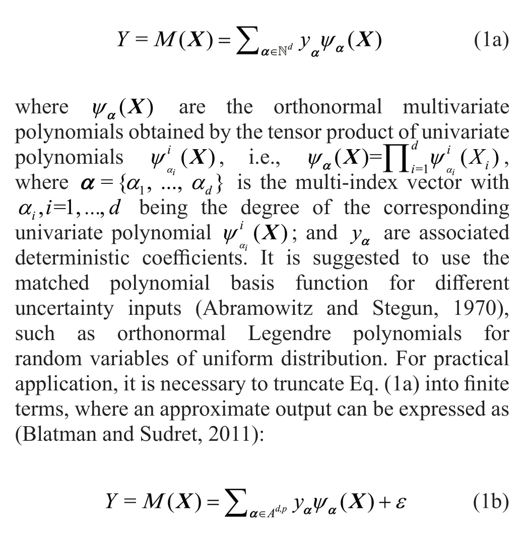
A structural system can generally be represented by a black-box modelMwith a few uncertain input variables that would affect its output. Typically, a number of uncertain input variables can be expressed in a vector form ofX={X1,X2,...,Xd}T∈Rd, wheredis the size of the vector; superscript T represents transpose; and each random variableXiis given a corresponding marginal probability density function, such as uniform, Gaussian, etc. The outputYof interest can be described as polynomial chaos expansion of the inputs:

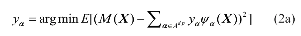
The coefficients usually can be obtained from the training set:

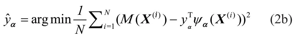
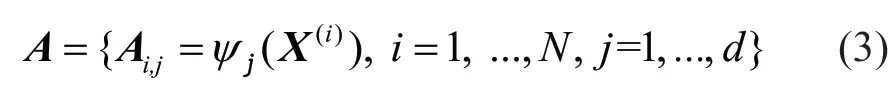
whereNgroups of different {X(1), . ..,X(N)} constitute the training set and each component is a single vector composed of uncertain input variables;is the corresponding response for the entire training set;Nis the size of the training set;ψα(X(i))={ψα1(X)(i),...,ψαp(X)(i)}is a vector containing the corresponding multivariate polynomials in the truncated basis, evaluated on thei-th set of the training sample. By estimating the polynomial onto each sample point in the training set, one can obtain the information matrix, which is defined as:

Equation (2b) represents a linear regression problem. Applying the least square solution leads to the coefficients as follows:

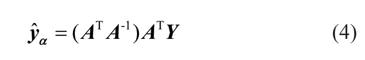
Using the coefficients from Eq. (4), accurate PCEs can be constructed to describe the dynamic response and to capture the propagation of uncertainty. The computational cost to solve the least square equation in Eq. (2b) is quite high, especially when high order polynomials must be used for high dimensional problems (Harikrishnan and Gupta, 2020). The accuracy of PCE can be improved by reducing the effect of over-fitting in least square regression. This can be achieved using sparse adaptive regression algorithms (Efronet al., 2004; Hastieet al., 2007). In particular, the least angle regression (LAR) algorithm (Blatman and Sudret, 2011) has been demonstrated to be effective in the construction of PCE. In this study, the MATLAB-based UQLab toolbox (Marelli and Sudret, 2014) is utilized for the realization of the sparse PCEs.

2.2 NARX Model

Generally, a dynamic system can be described by ordinary differential equations (continuous time) or difference equations (discrete time). For practical purposes, the dynamic process is discretized at discrete time instantst=1, …,Tto enable difference equations to represent the dynamic system. Following the law of causality, the current response or the state of a dynamic system is affected only by its previous states and external excitation signals (Mai, 2016). The NARX model, a well-known tool in system identification, can thus be defined as:

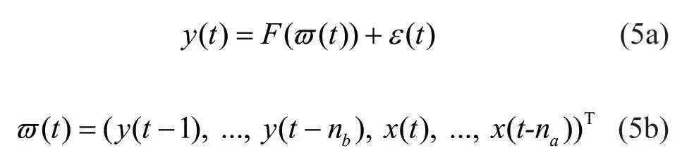
where ()tϖcontains all the regression terms incorporating current and past states;naandnbare the maximum time tags for excitation signals and structural response, respectively; ()Fis the performance function for the NARX model; and()tεis the residual error of the NARX model. Various global or local basis functions can be found in the literature to construct the regression terms in Eq. (5a), such as polynomials, splines, neural networks and wavelets. In this study, the following linear-in-the-parameters form is used (Chen and Billing, 1989):

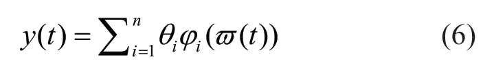
wherenis the number of model terms;ϕi(ϖ(t)) represents functions of regression terms; andiθis the corresponding coefficients. The NARX model provides a viable tool for describing the behavior of a dynamic system. To construct a precise NARX model, it is often necessary to account for the number of degrees of freedom, nonlinear behavior related to hysteresis, and geometry and mechanical properties, etc. This leads to a full NARX model, which usually contains more terms than needed for a proper representation of the dynamic system under consideration. Including these spurious terms in the model may result in numerical and computational problems. Therefore, Billings (2013) suggested identifying the simplest model to represent the underlying dynamics of the system. It is also reasonable to set the time tag to a limited value, considering that causality effects become increasingly weak between past states and the current state. Once the simplest NARX model is identified, the ordinary least squares algorithm will be utilized to obtain coefficients of the NARX model.

2.3 PC-NARX model

Uncertainties in a dynamic system play an essential role in its response. Consider a dynamic systemMas a generalized model to be expressed as:

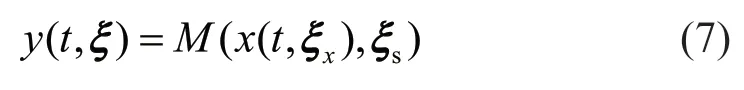
whereξ=(ξx,ξs)Tis the vector, composed of uncertain parameters;xξandsξrepresent the uncertainties in external excitation and the system itself, respectively. More specifically, vectorxξincorporates the parameters that control the frequency, duration and amplitude information of the external excitation, whilesξcan incorporate the parameters that affect system properties, such as geometries, stiffness, damping and hysteretic behavior. For the dynamic system represented in Eq. (7), Spiridonakos and Chatzi (2015) proposed integrating the PCEs and the NARX model to capture the propagation of uncertainty and to accurately describe responses of the dynamic system. Following the linear-in-theparameters form, the resulting PC-NARX model can be expressed as:

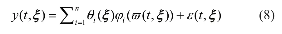
The PC-NARX model thus provides a framework where PCEs are used to capture uncertainty propagation through correlated NARX model coefficientsθi(ξ) (Soize and Ghanem, 2004) , which can be written as

whereε(t,ξ) is total error due to combining PCEs and the NARX model. It can be observed from Eq. (10) that there are two critical steps to construct an effective PCNARX model, i.e., constructing an adaptive NARX model and surrogate NARX coefficients through PCEs (Spiridonakos and Chatzi, 2015). However, not all the NARX and PC terms are adaptive for practice. For a full model that adequately considers knowledge acquired a priori, there exist redundant or computationally harmful terms, so that the use of this full model may result in large computational inaccuracy and therefore cannot establish an effective PC-NARX model (Mai, 2016). It is therefore important to identify adaptive NARX models and PCEs, i.e., to filter out redundant terms from NARX models.

2.4 NARX model selection

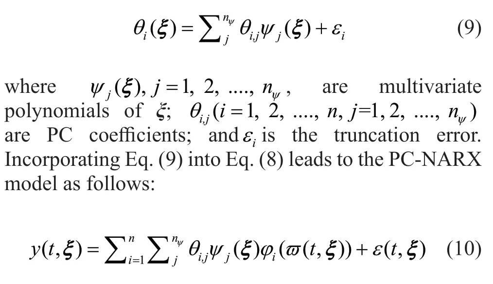
In order to filter out redundant terms out of a comprehensive full model, only structural responses exhibiting a high level of nonlinearity are concerned. In this study nonlinearity or maximum response values exceeding a specified threshold are used as measures to determine the training set for the PC-NARX model. A two phase method is introduced to construct the NARX terms and PC functions subsequently for the PC-NARX model (Mai, 2016). Fork-th experiment, the one-stepahead prediction of the response in the NARX model can be expressed as:

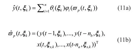
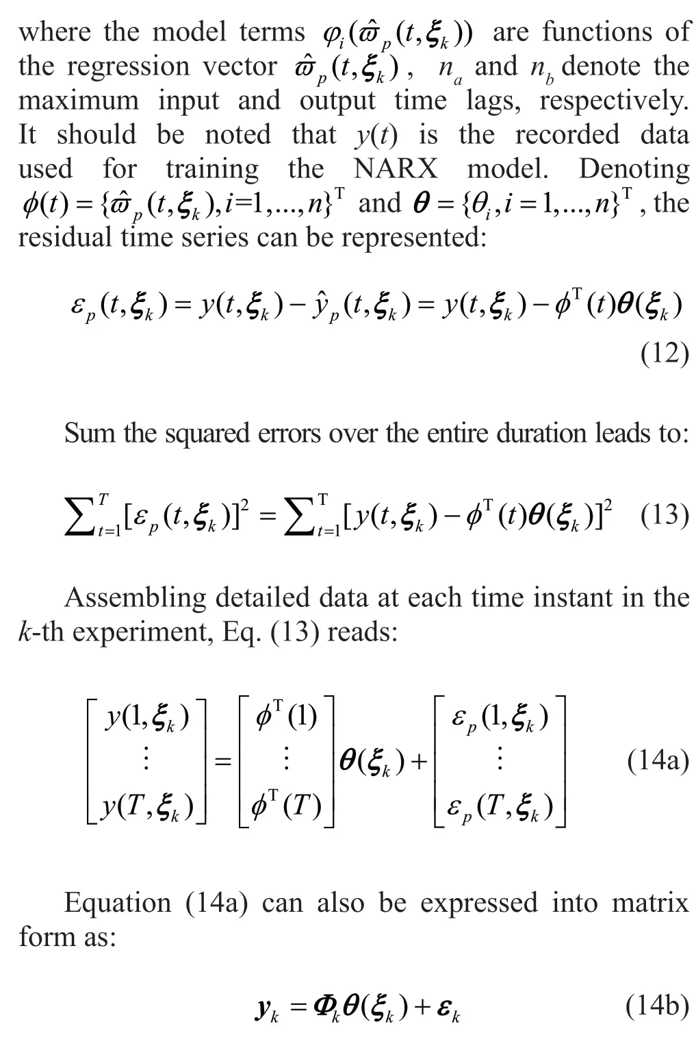
For each NARX model candidate, the corresponding NARX coefficients in Eqs. (14a) and (14b) can be derived for each of the training experiments using the ordinary least squares method. The minimization problem of Eq. (14a) can be expressed as follows:

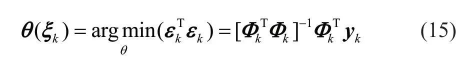
where the information matrixkΦcontains only the regressors specified in the NARX model candidate. Following the above procedure, NARX model candidates can be constructed for the entire training set. For a metamodel with the given initial response conditiony0, it is important to predict the dynamic response by using the following recursive form:

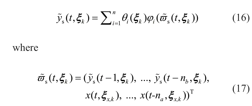
It can be observed from Eq. (16) that only the excitation signal seriesx(t) and the initial response0yare required for the prediction of the dynamic response, i.e., its estimate at one instant is used to predict the response at later instants. The relative error for thek-th simulation is stated as:

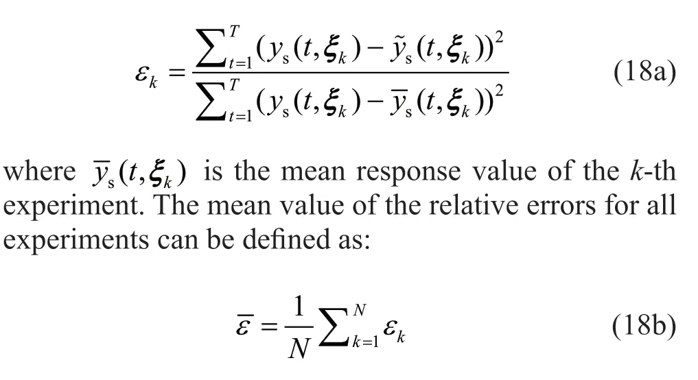
whereNis the size of training set; andkεis the relative error of thek-th experiment. The mean relative error in Eq. (18b) can be used to evaluate the accuracy of the model candidate. The model candidate with the smallest mean relative error is considered the most adaptive model.

Based on the above screening criterion, the task of screening the most adaptive candidate can be considered as a problem of feature selection, where various optimization algorithms can be found in the literature, such as particle swamp optimization (PSO), LARS and the GA algorithm. In this study, the GA algorithm is applied to search for the most adaptive model candidate (Spiridonakos and Chatzi, 2015). Each GA individual is a bit-string, with each bit representing the existence (1) or not (0) of the corresponding nonlinear term from the initial search space, also known as the full model. Starting from the GA solution, the nonlinear term whose removal has the minimum effect on the mean value of relative error is dropped, with the procedure being repeated till no more term is reduced. Figure 1 presents the flowchart to construct the PC-NARX model. Previous research has shown that the polynomial function basis helps construct the full model, i.e., a linear projection of trajectories on a deterministic basis. And it is also suggested thatnaandnbbe equal to twice the dynamic degrees of freedom. Moreover, when facing strongly nonlinear behavior, it has beens proved effective to introduce absolute response values to improve the accuracy in representation (Spiridonakos and Chatzi, 2015). Once the most adaptive NARX candidate is determined, its coefficients can be obtained by using the ordinary least square (OLS) method for all the experiments. These coefficients form the training set to be surrogated into the coefficients of the sparse PCEs.

3 Stochastic ground motion model

Stochastic ground motion model enables researchers to generate stochastic synthetic ground motions based on earthquake and site characteristics. In this study, the model proposed by Rezaeian and Der Kiureghian (Rezaeian and Kiureghian, 2008, 2010) is used to generate ground motion signals, where seismic ground motionx(t) can be represented by time-modulating a normalized filtered white-noise process with the filter having time-varying parameters as follows:

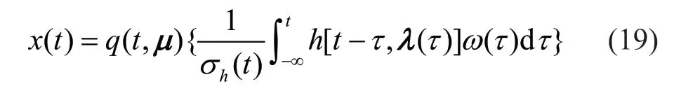
whereq(t,µ) is the deterministic and nonnegative time-modulating function, which completely defines the temporal characteristics of the process;ω(τ) is a white-noise process;h[t−τ,λ(τ)] denotes the impulseresponse function with time-varying parameters ()τλ; andσh(t) is used to normalize the standard deviation of the process. The modulating function can be expressed by three parameters controlling its shape and intensity as:

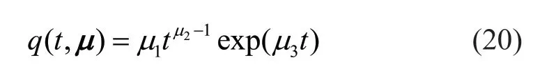
The vectorµ= (µ1,µ2,µ3)is related to three physically based properties, i.e., expected Arias intensityIaof the acceleration process, effective duration of the motion595D−and time at the middle of the strongshaking phase, i.e.,tmid. The impulse-response function has a form that corresponds to the pseudo-acceleration response of a single-degree-of-freedom linear oscillator as:

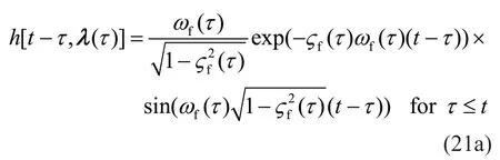
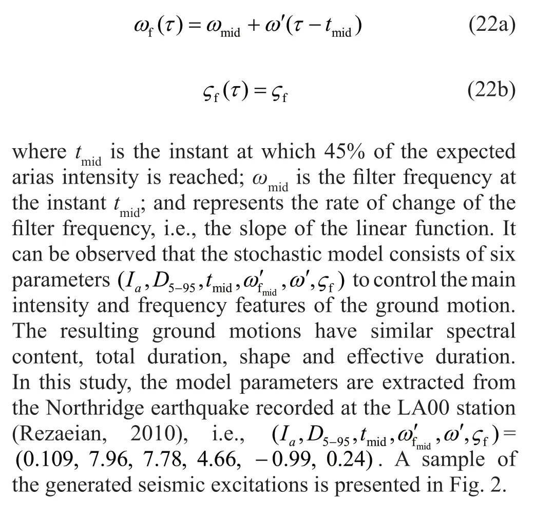
whereλ(τ)=(ωf(τ),ςf(τ)) is the vector of time-varying parameters of the filter;f()ωτandf()ςτdetermine the natural frequency of the filter and its damping ratio, respectively, and control the evolutionary predominant frequency and bandwidth of the process. In general, a linear form is selected forf()ωτand a constant value is forf()ςτ:

4 Generalized Bouc-Wen model with strength and stiffness degradation

It is widely accepted that response prediction can be a real challenge for a strongly nonlinear system with parameter uncertainties. This study aims to evaluate the sparse PC-NARX model for response prediction of a SDOF structure with nonlinear behavior involving stiffness and strength degradation. The Bouc-Wen hysteresis model (Baber and Noori, 1985; Wen, 1980) is used to incorporate the degradation into the dynamic equation of motion, which can be expressed as:

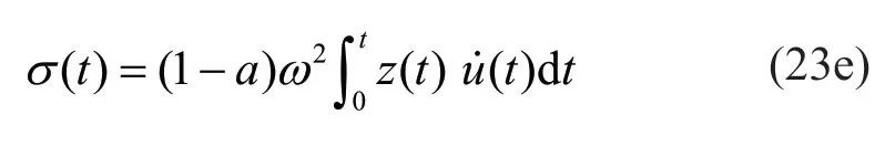
whereςis the damping ratio;ωis the fundamental frequency;ais the strain-hardening ratio;A,β,γ, andnare parameters to determine the hysteretic loops;v(t) andη(t) are the function governing the strength degradation and stiffness degradation, respectively;vδandηδare parameters controlling the rate of degradation; ()tσis the function describing hysteretic energy absorption, which is used to simulate degradation; ()utis the displacement; ()ztis the hysteretic term; and ()xtis the ground motion input.

For the purpose of analysis, three scenarios are considered, including strength degradation only, stiffness degradation only, and both strength and stiffness degradation. The degradation parameters for each of these scenarios are summarized in Table 1. Figure 3 presents typical hysteresis behavior of the Bouc-Wen model for the considered cases displayed in Table 1. Also presented in Fig. 3, for the purpose of comparison, is regular hysteresis behavior without strength or stiffness degradation. Strength and/or stiffness degradation can be observed to occur around a ductility demand of 2.0 in Figs. 3(a), 3(b) and 3(c), respectively. It is worth noting thatu/uyrepresents the ductility demand (normalized displacement) of the Bouc-wen model in Fig. 3, i.e.,uanduyare the displacement and the yield displacement of the Bouc-wen model. Similarly,f/fydefines the normalized force, i.e.,fandfyare the force and the yield force of the Bouc-Wen model. The other parameters of the generalized Bouc-Wen model are set to beζ= 0.02, 0a=,A= 1,n= 1,γ= 0. Thus, the parameter uncertainties for the SDOF structure can be considered mainly generating from an assembling vectorξ= (ω,β), as shown in Table 2.

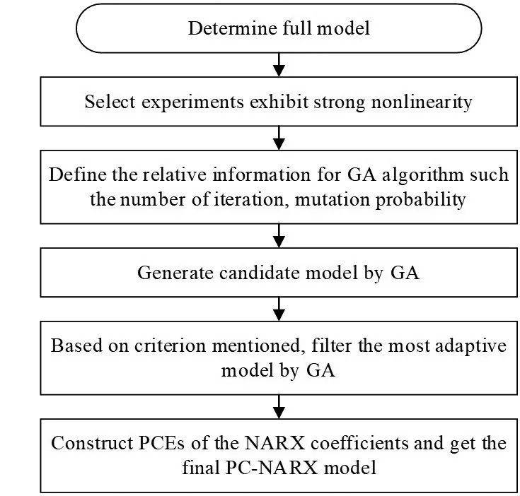
Fig. 1 Flowchart for constructing the sparse PC-NARX model

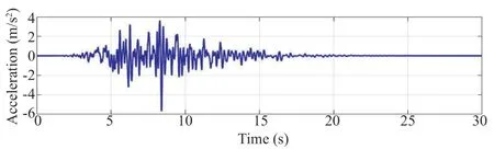
Fig. 2 Sample ground motion from the stochastic model

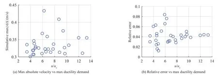
Fig. 4 Statistics of selected training sets for NARX model

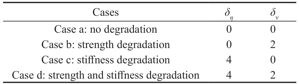
Table 1 Summary of three degradation situations

Table 2 Marginal distributions of the SDOF Bouc-Wen model

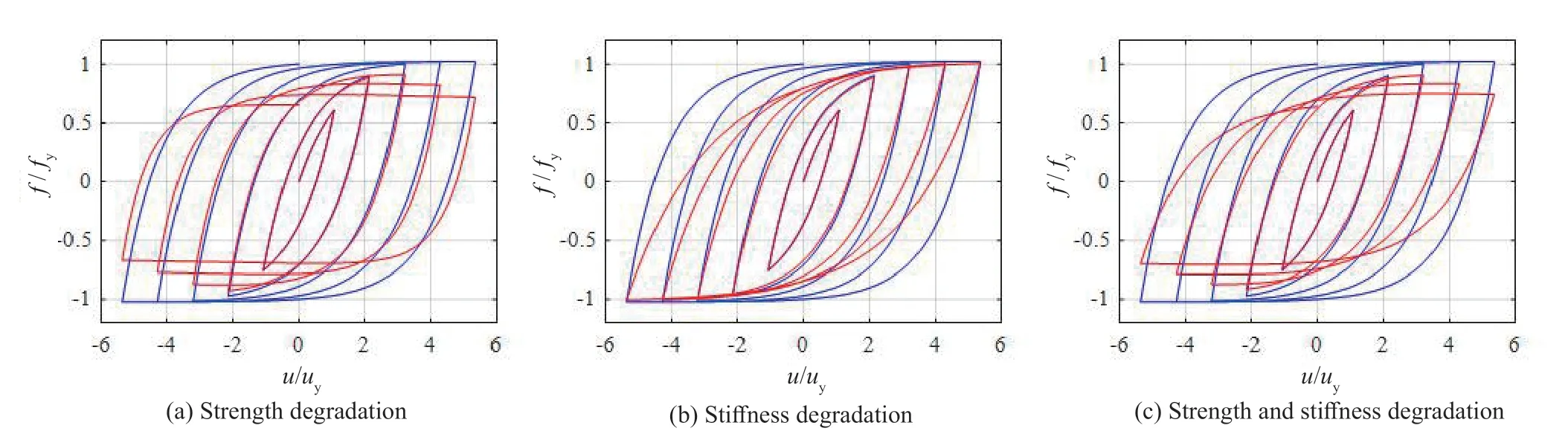
Fig. 3 Typical hysteretic behavior of Bouc-Wen models with stiffness and strength degradation

5 Response prediction using the PC-NARX model

5.1 NARX model selection results

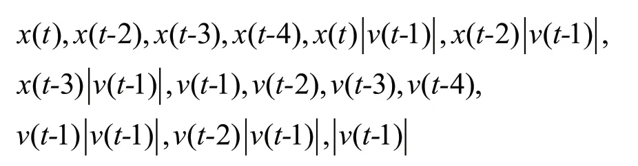
Velocity is selected as the target response in this study, as it is simpler to describe such a system by a single ordinary differential equation (ODE) with respect to velocity (Worden and Barthorpe, 2012). Fully considering prior knowledge about the system and excitation, the full NARX model, similar to that of Mai (Mai, 2016), is used in this study with the form:withl= 0, 1;m= 0, 1;j= 1, …, 4;k= 0, …, 4. Here,x(t) represents the ground motion input,v(t) represents the velocity of the structural system, i.e., ()ut˙ in Eq. (23a). The time tag used in this study is equal to four instead of two to accommodate the potential effect of strongly nonlinear behavior. This leads to a full model with a total of 20 terms, including the constant term. A total of 100 simulations of the nonlinear SDOF structure are used to select the terms of full model and to train the NARX model candidates for the three cases shown in Table 1. The uncertainty parameters are sampled by use of the Latin hypercube sampling (LHS) method (Helto and Davis, 2003). All ground motions from the stochastic model are set to 30 seconds for the purpose of comparison. The variable-step, variable-order (VSVO) Adams-Bashforth-Moulton method is used to solve the equation of motion in Eq. (18a) for the response of the nonlinear system with a total duration of 30 s and the time step of Δt= 0.005 s. The experiments with maximum absolute velocity exceeding a threshold were selected as the training set and this velocity threshold is set to 0.30 m/s, i.e., max(|v(t)|) > 0.30 m/s. Using these training sets, the GA algorithm is applied to search for the most adaptive NARX model candidate, with a minimum mean value of relative error. Sparse PCEs are then used to surrogate NARX coefficients to construct the final PC-NARX model. The optimal PCE order was found to bep=2 so that the resulting PC-NARX model leads to the smallest error. A total of 1000 simulations are further generated to validate the prediction results from the selected NARX model.

5.2 Response replication for SDOFs with stiffness degradation

For the SDOF with stiffness degradation, applying the threshold value for velocity response leads to 34 of 100 training sets. The minimum mean value of relative error is around 0.022, which implies that the final NARX model candidate was capable of accurate response replication for SDOF structures with stiffness degradation. The final selected NARX model includes the terms.

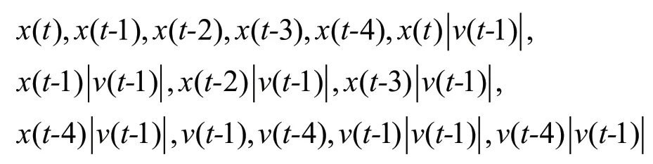
Figure 4(a) presents the statistics of maximum absolute velocity and maximum displacement ductility demand for these 34 training sets withmax(|v(t)|) > 0.30 m/s. It can be observed that most of the training sets have a maximum ductility larger than 4, with some extreme cases exceeding 12, indicating strongly nonlinear behavior. Figure 4(b) presents the relative error of the final NARX model with respect to the ductility demand for the 34 training sets. The relative errors are observed to be between 0.01 and 0.1, and not necessarily proportional to displacement ductility demand. Most of the training sets have a relative error around 0.04, implying that the final NARX model provides good accuracy in response replication of the SDOF structures when subjected to emulated ground motions.

A total of 1000 new simulations are generated to validate the PC-NARX model for response replication of the SDOF structure with stiffness degradation. The prediction time history of velocity can be obtained recursively by substituting the velocity and ground motion input of previous time points into the PCNARX model, of which the coefficients are determined from the uncertain parameter values. The displacement time history can also be obtained by integrating the corresponding velocity. Compared with traditional methods using an integration algorithm and a finite element program, the PC-NARX model provides an almost instantaneous solution, and is therefore extremely computationally efficient. Figures 5(a) and (b) compare the time histories of velocity and displacement responses between the computational simulation and the PC-NARX model prediction. Good agreement can be observed for both, indicating that the final PCNARX model provides an accurate structural response of the SDOF structure under investigation. Figure 5(c) presents the hysteresis behavior of the SDOF structure corresponding to the displacement response in Fig. 5(b). Stiffness degradation can be observed with displacement ductility close to 4.

Fig. 5 Comparison between simulation and PC-NARX prediction for the SDOF system with stiffness degradation

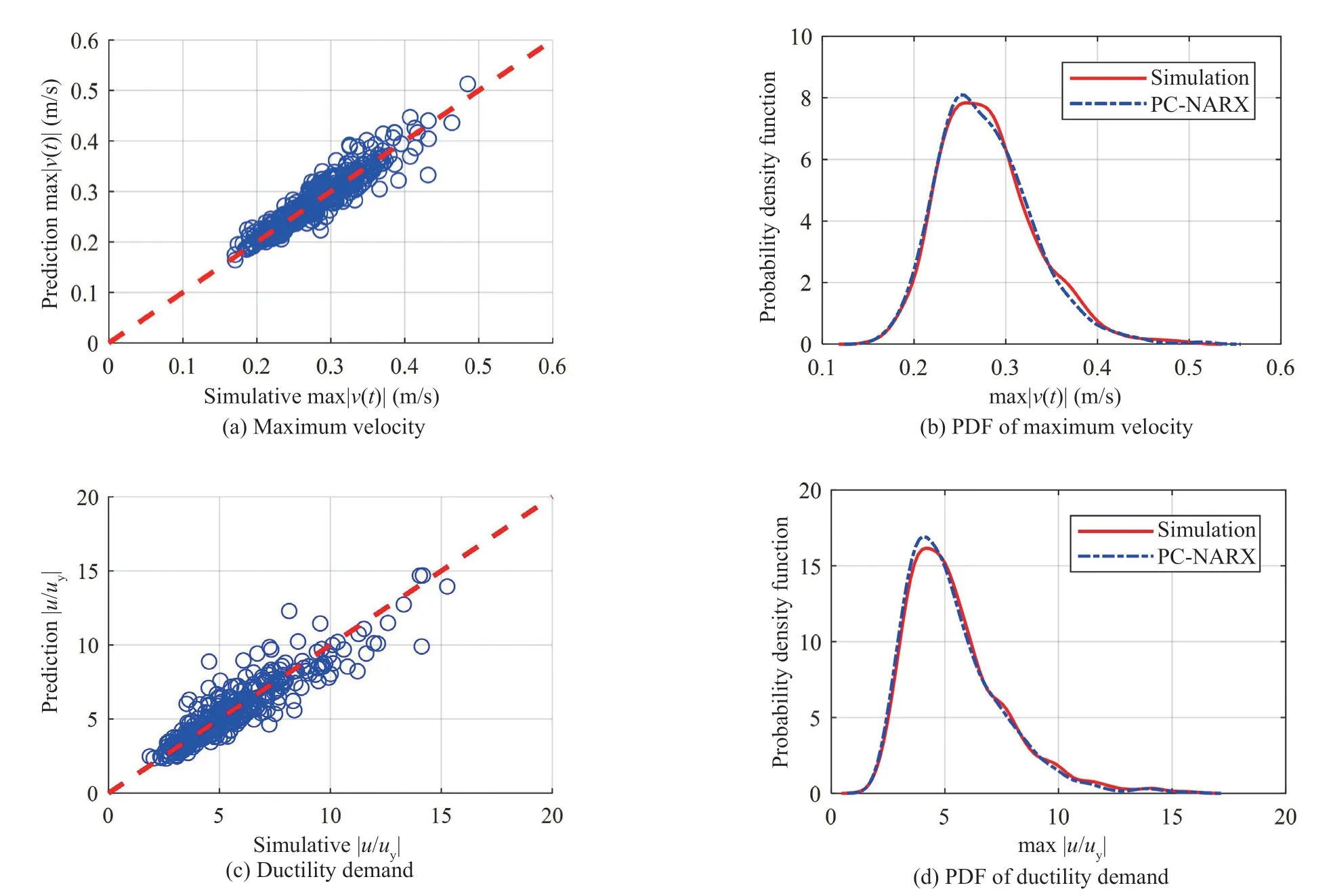
Fig. 6 Prediction for maximum velocity and ductility demand for the SDOF system with stiffness degradation

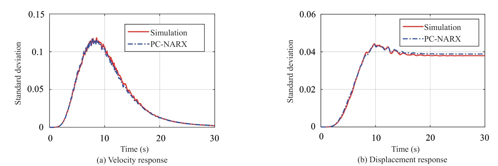
Fig. 7 Standard deviation of velocity and displacement response

Fig. 8 Statistics of selected training sets for the NARX model

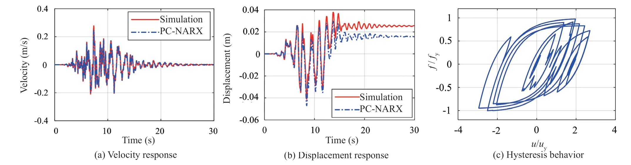
Fig. 9 Comparison between simulation and PC-NARX prediction for the SDOF system with stiffness degradation

To statistically evaluate the capability of the PCNARX model for response replication, Figures 6(a) and 6(c) compare the maximum velocity response and displacement ductility demand, respectively, between the computational simulation and the PC-NARX model prediction. It can be observed that predictions from the PC-NARX model are very close to those from numerical simulation for almost all the validation sets. Even for the cases with maximum velocity or ductility demand larger than those of training sets, the PC-NARX model also shows good accuracy. Figures 6(b) and 6(d) present the probability density functions (PDFs) of the maximal absolute velocity and the ductility demand, respectively. Overall, accuracy of the prediction can be considered good in most predictions for a wide range of values for maximum absolute velocity and ductility demand. This again proves the statistical accuracy of the response predicted by the PC-NARX model for strongly nonlinear structures.

The statistical moment is used to further verify the accuracy of the PC-NARX model. Figure 7 presents the standard deviation of the velocity and displacement responses over the duration of ground motion, where good agreement is observed between the computational simulation and the PC-NARX model prediction. This again proves the accuracy and effectiveness of the PCNARX model for response prediction of the SDOF structure with stiffness degradation.

5.3 Response prediction for SDOFs with strength degradation

For the SDOF structure with strength degradation, applying the threshold value of max(|v(t)|) > 0.30 m/s leads to 27 of 100 training sets. The minimum mean value of relative error is around 0.0025. The final NARX model includes the terms

and the constant term. Figure 8(a) presents the statistics of maximum absolute velocity and ductility demand for the selected 27 training sets. Similar observations to those displayed in Fig. 4(a) can be made in Fig. 8(a), namely, that most ductility demands fall between 4 and 10, for a good representation of strongly nonlinear behavior. Figure 8(b) presents the relative error of the final NARX model with respect to the ductility demand of the 27 selected training sets. The relative errors are observed smaller than 0.06, implying good accuracy in the final PC-NARX model.

For the 1000 new simulations to validate the final PC-NARX model, Fig. 9 compares structural responses between the numerical simulation and the PC-NARX model prediction for a range of input parameters. Good agreement can be observed for the comparison of velocity response shown in Fig. 9(a). Although slight discrepancies are observed for the residual deformation, as can be seen in Fig. 9(b), the PC-NARX model is observed for good prediction of peak displacement. The recursive prediction of the PC-NARX model often has errors that accumulate continuously throughout the time duration, eventually leading to larger errors for a quite strong nonlinear system. Figure 9(c) shows the hysteresis behavior with strength degradation.

Figure 10 compares the maximum structural response quantities and their PDFs between the computational simulation and the PC-NARX model prediction, including the maximum velocity response appearing in Fig. 10(a) and the displacement ductility demand shown in Fig. 10(c). It can be observed that predictions from the PC-NARX model match very well those from numerical simulation for almost all the validation sets. Figures 10(b) and 10(d) present the PDFs of maximal absolute velocity and ductility demand. It can again be observed that PDFs of the computational simulation and the PC-NARX model prediction match each other well. This implies that the PC-NARX model provides good statistical accuracy for the nonlinear SDOF with strength degradation.

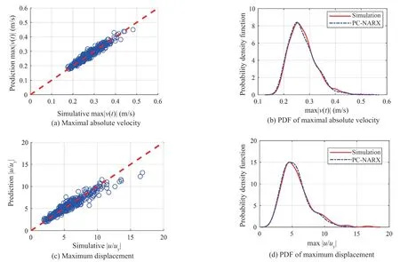
Fig. 10 Prediction for maximum velocity and displacement responses for SDOFs with strength degradation

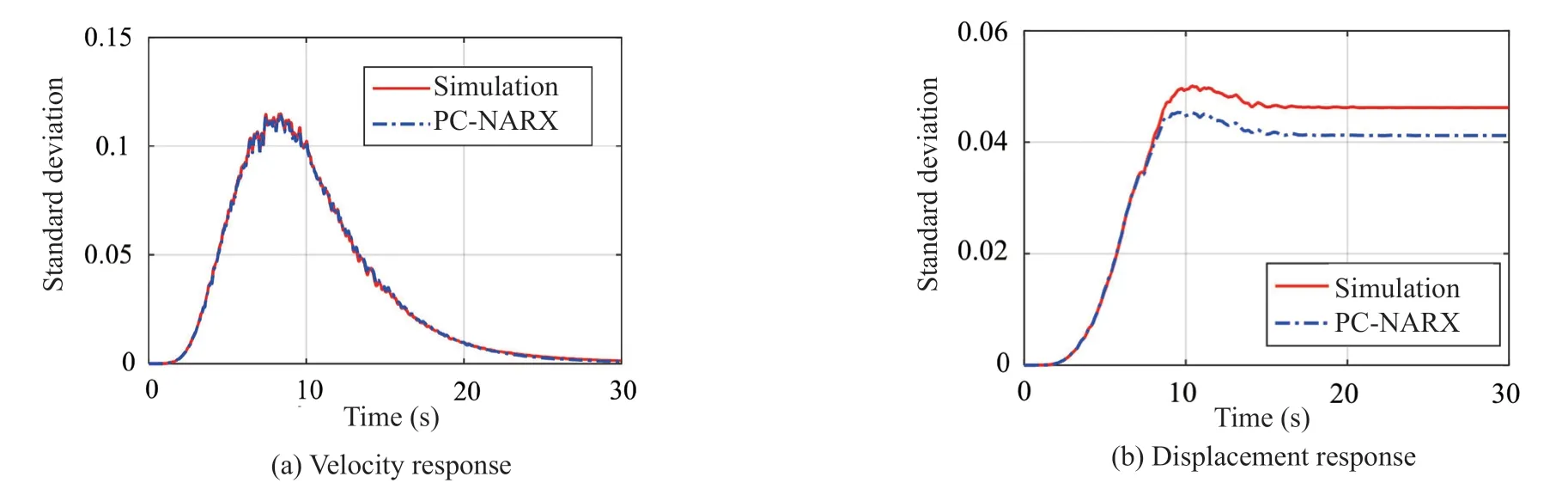
Fig. 11 Standard deviation of the PC-NARX model

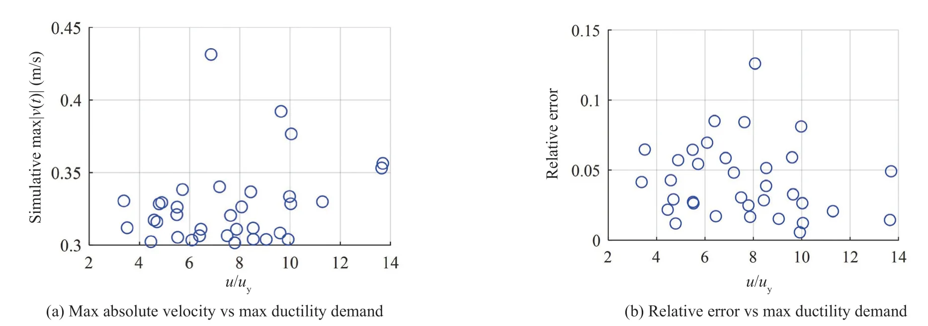
Fig. 12 Statistics of selected training sets for the NARX model

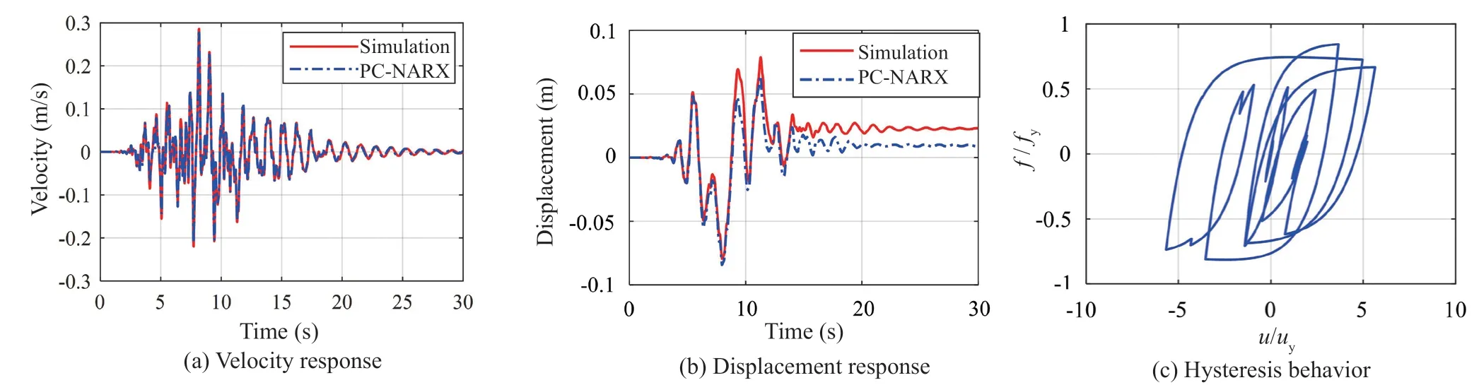
Fig. 13 Comparison between simulation and PC-NARX predictions for SDOFs with stiffness and strength degradation

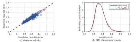
Fig. 14 Prediction for maximum velocity and displacement responses for the SDOF system with stiffness and strength degradation

5.4 Response prediction for SDOFs with both stiffness and strength degradation

For SDOFs with both stiffness and strength degradation, applying the threshold value for velocity response leads to 34 out of the 100 training sets. The minimum mean value of relative error is around 0.0024. The final NARX model has the terms of

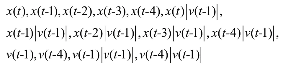
Figure 12(a) presents the statistics of maximum absolute velocity and displacement ductility demand for the thirty-four training sets. It can be observed that the displacement ductility falls between 4 and 10, implying that these training sets provide good coverage of nonlinear behavior. Figure 12(b) presents the relative error of the NARX model with respect to the displacement ductility demand for the 34 training sets. The value of relative error is observed independent of the ductility and almost all values of relative error are less than 0.1.

Figure 13 compares structural responses between the computational simulation and the PC-NARX model prediction for the SDOF structure under a set of uncertainty parameters. Good agreement is again observed for the velocity however slight discrepancy for the displacement response, which is obtained by integration of corresponding velocity over time. The difference in displacement can be attributed to the cumulative error in the velocity. The hysteresis behavior of the SDOF structure corresponding to the response in Figs. 13(a) and 13(b) is presented in Fig. 13(c). Both stiffness and strength degradation can be observed.

For the 1000 validation simulations and the PCNARX model prediction, Fig. 14 compares the maximum structural responses quantities and their PDFs, including the maximum velocity response in Fig. 14(a) and the displacement ductility demand in Fig. 14(c). It can be observed that predictions of velocity responses from the PC-NARX model have better accuracy than those of displacement responses. Same observation can also be made for the PDFs of maximal absolute velocity and ductility demand in Figs. 14(b) and 14(d). The PC-NARX model provides good statistical accuracy for the nonlinear SDOF with both stiffness and strength degradation.

The comparisons of statistical standard deviation over the time duration are presented in Fig. 15, where the standard deviation of the velocity response is nearly perfectly matched. Similar to Fig. 11, slight discrepancy is observed in the standard deviation of the displacement response. This implies that the stiffness and strength degradation together reduce the accuracy for displacement prediction of PC-NARX model.

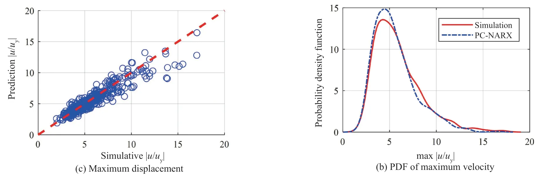
Fig. 14 Continued

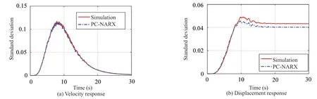
Fig. 15 Standard deviation of response

6 Summary and conclusions

To better predict structural responses close to collapse, the PC-NARX model is explored in this study for response prediction of SDOFs with stiffness and/or strength degradation. Using selected uncertainty parameters, the PC-NARX model is established based on training sets used in this study, then evaluated for validation sets for SDOFs with stiffness and/or strength degradation. Time histories of structural responses are compared for both displacement and velocity. More specifically, statistical standard deviation is also used to validate the accuracy of the PC-NARX model prediction in addition to the maximum absolute velocity and the displacement ductility demand, as well as their PDFs. Generally, the PC-NARX model demonstrates good accuracy for response prediction of SDOF structures with significant stiffness and/or strength degradation. Through the use of the PC-NARX model, structural response can be obtained with significantly less computational cost when compared to conventional time history analysis. Uncertainty in the SDOF structures can be well accounted for through the subrogation of NARX model coefficients. However, determination of an optimal NARX model from training sets is found to be very time consuming, which could make the search of best model candidate a significant challenge for more realistic structures. It is also shown that degradation due to strongly nonlinear behavior could slightly influence the accuracy of PC-NARX model prediction, especially for displacement responses. Compared with stiffness degradation, strength degradation is observed to be statistically more influential on the accuracy of the PCNARX model. Overall, the results presented herein demonstrate that the PC-NARX model is a promising, reliable and robust approach for nonlinear response prediction of structures close to collapse. Evaluation of the PC-NARX model for more realistic structures close to collapse is currently under investigation and will be reported on in a future publication.

Acknowledgement

This research was financially supported by the National Natural Science Foundation of China under Grant No. 51878390. The authors wish to acknowledge the sponsors. However, any opinions, findings, conclusions and recommendations presented in this paper are those of the authors and do not necessarily reflect the views of the sponsors. Finally, yet importantly, the authors wish to thank the three anonymous reviewers for their careful evaluations and insightful comments that helped improve this paper.