A Novel Product Remaining Useful Life Prediction Approach Considering Fault Effects
2021-10-23JingdongLinZhengLinGuoboLiaoandHongpengYin
Jingdong Lin,Zheng Lin,Guobo Liao,and Hongpeng Yin
Abstract—In this paper,a novel remaining useful life prediction approach considering fault effects is proposed.The Wiener process is used to construct the degradation process of single performance characteristic with the fault effects.The first passage time based remaining useful life distribution is calculated by assuming fault occurrence moment is a random variable and follows a certain distribution.Expectation maximization algorithm is employed to estimate model parameters,where the fault occurrence moment is considered as a missing data.Finally,a Copula function is used to describe the dependence between the multiple performance characteristics and derive joint remaining useful life (RUL)distribution of product with the fault effects.The effectiveness of the proposed approach is verified by the experiments of turbofan engines.
I.INTRODUCTION
REMAINING useful life (RUL)prediction is a key technology of ensuring the product’s reliability and safety,it is also an effective path to reduce the maintenance costs for practical product [1],[2].Therefore,the researches on the RUL prediction methods have drawn much attention from both academia and engineering circles in recent years.In general,RUL prediction means to find the probability distribution function (PDF)of the RUL or the expectation value of the RUL [3],[4].Most of products have their own performance characteristics (PCs)that increase or decrease over time,and PCs are collectively referred to as degradation data.As degradation data is directly related to the health condition of the products,the prediction methods based on degradation data become more and more popular [5]–[8].
In past few decades,there are many methods of RUL prediction based on degradation data that have been researched,these are generally summarized into three types:physical,data-driven,and hybrid methods [9].Among these categories,the methods of data-driven become the mainstream direction in research of RUL prediction,because the methods only need to establish a statistical model to fit the observations without any assumption of physical parameters or additional expertise.Machine learning has been extensively studied in the past decade,it does not need to understand the degradation mechanism of the product,but uses a large amount of data to train the prediction model.In order to improve the accuracy of remaining life prediction,Gebraeel and Lawley [10] were the first to use the trained neural network to calculate the remaining life distribution function of the device based on the monitored data.Renet al.[11] used the self-encoding multidimensional feature extraction to characterize the health degradation trend of the battery,and then trained the life prediction model based on the deep neural network,and successfully applied the method to the prediction of the remaining life of the lithium battery.Wuet al.[12] used the least squares support vector machine (SVM)method to fit the performance degradation process of equipment for the problem of only a small number of samples in reliability analysis.Tranet al.[13] used the minimum mean variance to establish a degenerated index of equipment,and then used the established index as training data to complete the remaining life prediction test of related mechanical equipment by combining with SVM.However,because of random and dynamic characteristics of product’s degradation process,the stochastic-process based prediction approaches have attracted great attention in the data-driven methods.According to Siet al.[14],the data-driven based RUL prediction methods are classified into two main types:indirect data and direct data based methods,and the scope of application of stochastic process in the prediction of RUL is illustrated in detail.The stochastic process mainly includes Markov chains,Wiener processes,and Gamma processes.Among them,for its important physical interpretation and nice mathematical properties,Wiener process can describe non-monotonic degradation process of many typical products.It has been widely applied to establish the degradation process and predict the RUL of a variety of industrial components.Tsenget al.[15] used a Wiener process to determine the lifetime for the light intensity of light emitting diode (LED)lamps of contact image scanners.The Wiener process was even extended to the adaptive Wiener process model by Zhai and Ye [16].More detail about Wiener process applied in RUL prediction can refer to [17].
In reality,many products usually have complex structure,and consist of multiple components or a component having multiple PCs.Compared to single PC,multiple PCs can provide more accurate information for RUL prediction.In such a situation,a bivariate or multivariate degradation model is needed to estimate RUL of products,where the existing methods can be roughly classified into multivariate distribution,multivariate stochastic process and Copula function.Multivariate normal distribution as a popular method has been utilized to identify a multivariate joint probability[18].Wang and Coit [19] conducted a degradation analysis of a system with multiple degradation measurements,and introduce a multivariate s-normal distribution model.Multivariate or bivariate degradation process models based on Gamma processes,Wiener processes are introduced by[20]–[23].In practice,assuming degradation data follows a multivariate distribution or multivariate stochastic process may not be suitable for all conditions,when degradation mechanisms of multiple PCs are not consistent or independent.As a useful alternative,Copula function is employed to identify a multivariate joint probability [24].Due to its flexibility,Copula function has been widely used in RUL prediction of a product with multiple PCs.Sariet al.[25] investigated the degradation mechanisms of LED lamps,and presented a bivariate degradation model based on Copula function.Copula function is widely applied in degradation modeling,reliability analysis and prognostics,more introductions are in [26]–[29].
In practice,with the wear of the components,overload operation,or the changes of environment factors,many different kinds of faults may occur in the product’s degradation process.Most of these faults are not equal to the functional failure,product can continue to work,but the occurrence of the fault will aggravate its degradation degree and change the product’s degradation trajectory,ultimately shorten the product’s RUL.Meanwhile,there are many researches about that some product’s degradation path will be changed at a moment and even more times during the degradation process.More specially,after a product has degraded down to a certain level (which can be called transition time),the initial function form of the condition monitoring signal may be changed,evolve more rapidly or gradually compared to the early stage of usage.It is a quite common phenomenon that degradation trajectory changes during the degradation process for display devices,such as plasma display panels,LED,and organic light emitting diode(OLED)studied by Tanget al.[30] and Ng [31].Siet al.[32],research the RUL prediction of systems with operation state switching between the working state and storage state,and the degradation rates of two states are different,the transition time and transition number are derived.Cuiet al.[33] assumed that the changing location was determinate,and the Wiener process is employed to model the degradation process,the first passage time of the degradation process governed by a discontinuous trend function is studied.
However,the fault is hard to be detected,if it occurs after observations,it means the fault may not occur in observations but in a future span,and its probability of occurrence increases over time.Therefore,compared to the operation state switches and determinate changing location,the transition time from normal state to fault state (which can be called fault occurrence moment (FOM))is difficult to be detected directly,so the changing time of the degradation rate with the fault effects is unobservable and random.The effects of a fault in the degradation process cannot be neglected,because the occurrence of FOM will accelerate the failure of the product.Moreover,very few efforts have been made to address the RUL prediction which involves fault effects.Besides,when a fault occurs in the degradation process,the degradation rates of multiple PCs will be changed at the same time,which is shown in Fig.1.In addition,PCs may be dependent because of the strong coupling between the product’s components.Therefore,our final goal is to estimate the RUL joint distribution of multiple dependent PCs considering fault effects.
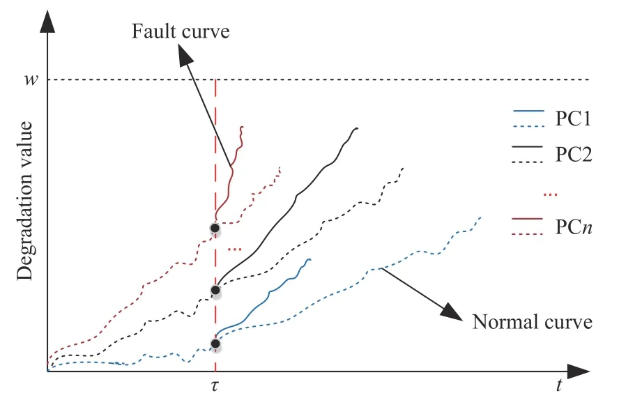
Fig.1.The degradation process of multiple performance characteristics for two states.
In this paper,in order to solve the problem of the product RUL prediction with the fault effects,the proposed approach is divided into two parts.First,a degradation model based on the Wiener process is used to account for the changing of degradation process.In the presented model,the drift coefficient is utilized to describe the fault effects for the whole degradation path,and the diffusion coefficient characterizes the stability of the degradation process respectively.Then,the RUL distribution of the product based on the definition of first passage time is obtained,where it is assumed that FOM is a random variable and follows a certain distribution.In this work,the FOM is regarded as a missing-data in the observations since the FOM can not be detected directly,expectation maximization (EM)algorithm is employed to tackle the problem of parameter estimation.Then,the product RUL for single PC considering fault effects can be estimated.Second,as multiple PCs will be influenced by the fault at the same time,and may be dependent during the degradation process.A Copula function is used to describe the dependence between multiple PCs and derive the RUL joint distribution of the product based on the RUL distribution of single PC with the fault effects.
The main contributions of this paper are summarized as follows:
1)A novel product RUL prediction approach is proposed for the problem that degradation process is impacted by the fault effects,which considers the FOM as a random variable and follows a certain distribution.To the best of our knowledge,this is the first time to consider fault effects into the RUL prediction.
2)As FOM cannot be detected directly after observations,which causes the incomplete observations,FOM is regarded as a missing-data in problem of parameter estimation.EM algorithm is used to estimate parameters of degradation model and fault distribution simultaneously.
3)For the multiple PCs will be affected by the fault and may be dependent during the degradation process,Copula function is employed to describe the dependence of PCs and obtain the joint distribution function of the product’s RUL.
The rest of this paper is organized as follows.In Section II,the degradation model based on the Wiener process is established considering fault effects.RUL distribution is discussed in Section III.Section IV focuses on the method of inference for the unknown parameters.The RUL prediction of product with multiple PCs that are influenced by fault is given in Section V.The experiments and results analyses are given in Section VI to illustrate the effectiveness accuracy of the proposed method.Finally,some concluding remarks and discussions are made in Section VII.
II.DEGRADATION MODEL WITH FOM FOR SINGLE PC
As a mathematical expression of Brown motion (BM),Wiener process has been widely used in degradation modeling.Consider single fault occurs in the degradation process,which can be described by changing the drift parameter of Wiener process.In this section,we focus on the degradation process models governed by the Wiener process considering fault effects.In general,a Wiener process based degradation model can be represented by

where λ is a drift coefficient,σ is a diffusion coefficient andB(t)is a standard BM,B(t)∼(0,t),X(0)represents the initial value of the degradation process.Without loss of generality,X(0)is zero,soX(t)∼N(λt,σ2t).
1)Continuous Degradation Model Considering Fault Effects
Equation (1)demonstrates a normal degradation process,but through the above analysis in Section I,the fault may be generated during the degradation process,so the product suffers additional load,and this state has a higher degradation rate than the case in the normal state.The FOM separates the whole degradation process into two states,the former is a gradual degradation state expressed and the latter one is a rapid degradation state.Therefore,the whole process can be described by changing drift function,the diffusion coefficient σis assumed to be the same during the both states.The degradation process considering fault effects is then indicated as

where τ is the FOM,λ1and λ2are the degradation rates fort<τ andt≥τ,respectively.X(t)is normally distributed asX(t)∼N(λ1t,σ2t)fort∈[0,τ)andX(t)∼N(λ2(t−τ)+λ1τ,σ2t)fort∈[τ,+∞).
2)Increment Degradation Model Considering Fault Effects
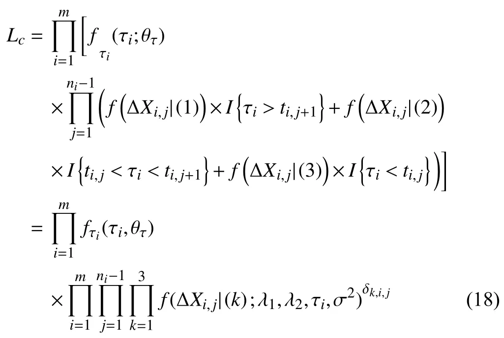
As the measurement time is discrete,we suppose thatmsimilar products are tested,andXi,jdenotes the degradation observation value of performance characteristics for productiat timeti,j,{i=1,...,m;j=1,2,...,ni},whereniis the number of inspection time of each product.∆Xi,j=Xi,j+1−Xi,jfrom∆ti,j=ti,j+1−ti,j.The increment degradation model considering fault effects can be divided into three cases.
Case 1:(τ≥ti,j+1)

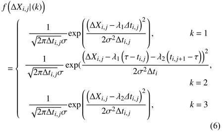
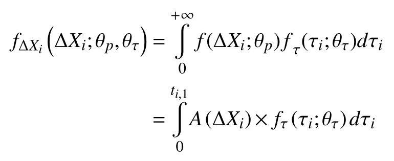
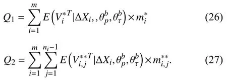
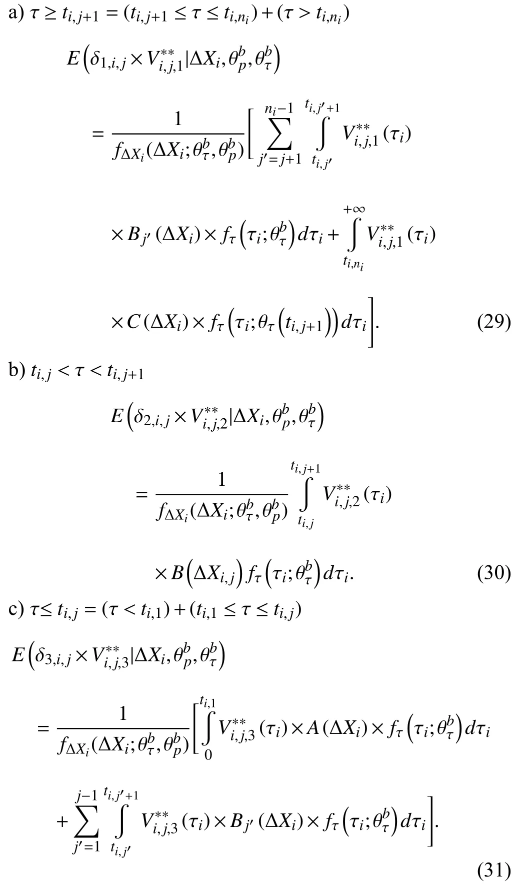
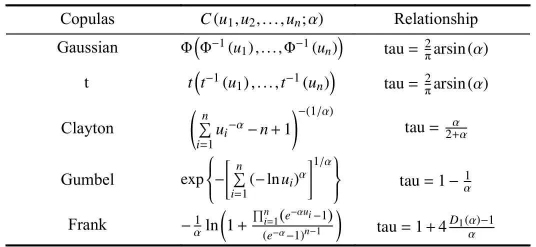
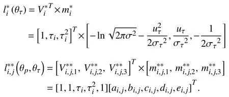
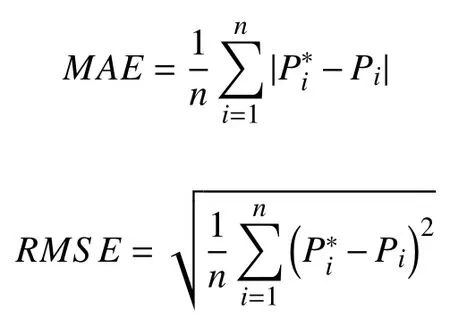
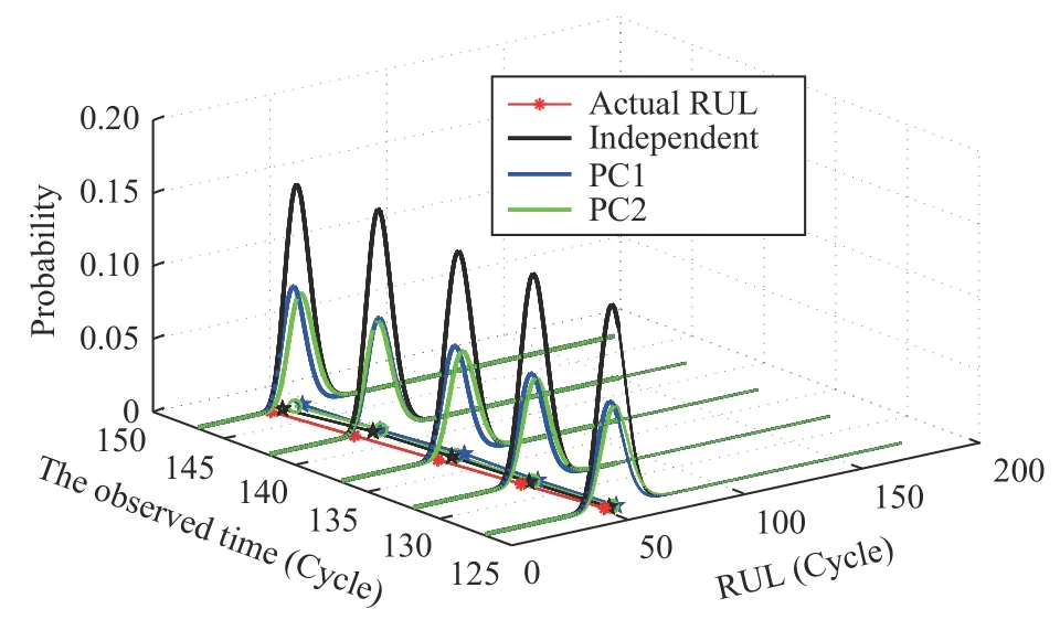
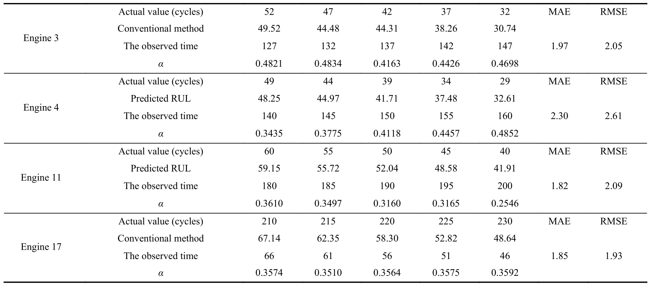
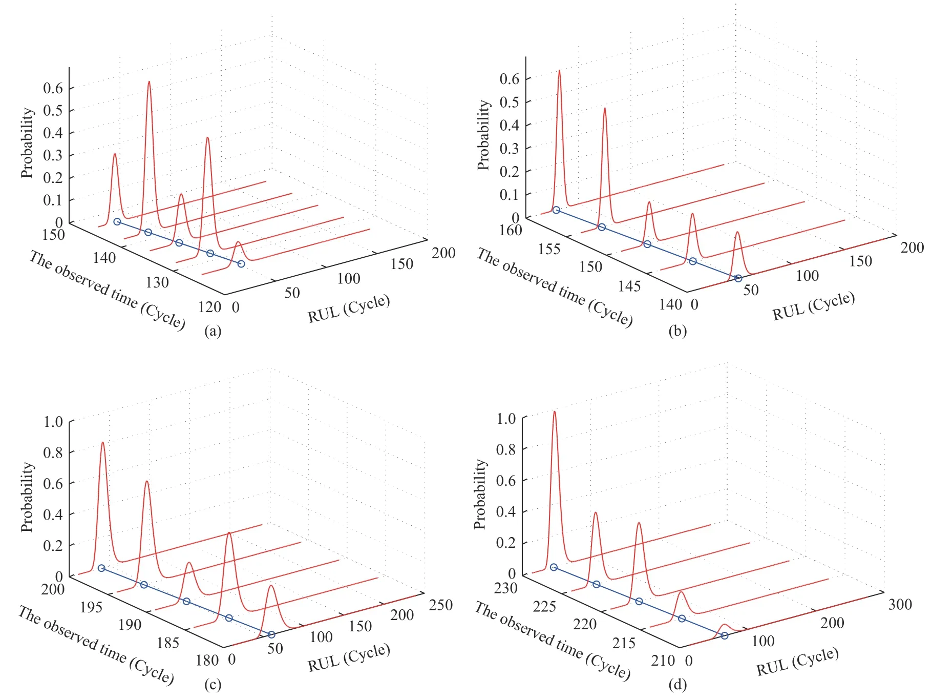
Case 2:(ti,j<τ Case 3:(τ≤ti,j) where three cases respectively represent the FOM occurs after the increment,FOM occurs in the increment,FOM occurs before the increment. According to specifications above,the PDF of the increment∆Xi,jis expressed as wherek=1,2,3 denote the scenarios τ>ti,j+1,ti,j<τ Here,our attention is paid on not only the degradation model for single PC considering fault effects,but also RUL distribution and parameter estimation.Therefore,two important parts in the following sections are described in detail. In general,the prediction for product’s RUL often means to find its PDF or cumulative distribution function (CDF)of RUL distribution and calculate the expectation value finally.Therefore,one of the main goals is to obtain RUL distribution for the product.Based on the concept of the first passage time,a product is regarded as to be failure,when its degradation value exceeds the preset failure threshold.Supposewis the failure threshold,andXi,jhas not exceeded the failure thresholdw.The lifetimeTunder the concept of the first passage time is expressed as Therefore,letLi,jdenote the RUL at timeti,jas wherelis the time interval of a product that from normal state to failure state. At first,consider the degradation process without the fault.According to properties of the Wiener process,the CDF of RUL in the normal state follows the inverse Gaussian distribution where Φ(·) is a standard normal distribution,Zi,jrepresents current observation value at observation timeti,j. The corresponding PDF is However,the degradation process in (2)is divided into two parts by FOM τ.The PDF of RUL distribution should also consist of two parts,and if the FOM is determined and its position is known in observations,the PDF can be expressed as where 0 Because the FOM is unobservable in the future,it is impossible to know its precise position,so form (11)is not applicable.To derive the RUL distribution,the FOM is regarded as a random variable which is assumed to follow a certain distribution,and the CDF and PDF of the FOM aref(τ;θτ),F(τ;θτ),respectively,where θτis the set of unknown parameters of distribution function.The CDF of RUL distribution can be then expressed as According to above specification,the unknown parameters considering fault effects consist of θp={λ1,λ2,σ} and θτ.In this section,we focus on the issue of parameter estimation under the assumption that the FOM is a random variable.FOM τ cannot be observed in the future span,this will cause the incomplete observations,and the FOM is regarded as a missing data in the observations.In a missing-data problem,EM algorithm is used to estimate the parameters θp,θτ.The EM algorithm consists of two steps performed iteratively.The expectation-step (E-step)computes the expectation of the loglikelihood with respect to the complete-data conditioned on the observed data.The maximization step (M-step)then finds the maximizer of this expected likelihood [31].The two steps are repeated iteratively until satisfactory convergence is achieved. For applying EM algorithm,observed data likelihood needs to be obtained firstly.Let {τ1,τ2,...,τm} be the FOM set corresponding tomproducts which are random variables during the degradation process of each product.Because the FOM is random in the degradation process,the joint PDF of increment for each product ∆Xiis then written in three cases: 1)Fault occurs before all observations (τi 2)Fault occurs in observations (ti,1≤τi≤), 3)Fault occurs after all observations (<τi), The joint PDF of ∆Xiconditioned on τiforith product is then expressed as Observed data likelihood is then written as The PDF of τ is given,and the complete data vector consists of {∆X,∆t,τ},where τ is a set of the FOMs{τ1,τ2,...,τm},the complete-data likelihood is where δk,i,jis an indicator variable for τ and ∆ti,jin three scenarios,such as when scenariok=1,2,3 occurs,it corresponds to the δk,i,j=1,k∈1,2,3,δk,i,j=0 otherwise. The complete-data log-likelihood is then written as Use the following notation for simplifying the above loglikelihood expression The complete-data log-likelihood can then be written as In order to apply the EM algorithm to solve the maximum likelihood estimates of (λ1,λ2,σ2)for the case that the FOM is not observed,the problem is firstly cast as a missing-data problem,whereτ is regarded as the missing data in observations. 1)E-step:The goal of the E-step is to compute the expectation of the complete-data log-likelihood of the missing-data conditioned on the observed data ∆X,∆t. The EM algorithm is only effective for the case that the complete-data likelihood is linearly separable in the set of missing-data statistics,and form (23)is not analytical-form.Therefore,the missing data τ from the function needs to be separated,log-likelihood expression can be written in the form of=VT·m∗,where the vectorVconsists of only functions of the missing data τ,andm∗consists of only θp,θτand observe data.In the forms,the components of the loglikelihood expressions are,where So,m∗consists ofand,Vconsists ofand.When linear separability can be established,it is then necessary to compute the expectations ofVconditioned on observed data.FormQ1andQ2given in (23)can be expressed as respectively The conditional expectation forcan be evaluated as follows: Next,the conditional expectation under the second summation series given in (23)is computed.However,it involves conditional expectation of δk,i,j·,which needs to be discussed in three cases: 2)M-step:Based on E-step,updateb=b+1,new estimates for θbcan be generated by solving for the complete-data MLE to (23).AsQ1only contains θτandQ2only contains θp,the estimator vectorsandcan be calculated by (32),(33),respectively. One iteration is completed throughMsteps,repeat the above two steps so that when the parameters tend to converge or the number of iterations is reached,the iteration will be stopped. The RUL prediction of the product with single PC considering fault effects can be calculated by Sections II-IV.As the occurrence of the fault can change the degradation trajectories of multiple PCs,the final goal is to obtain RUL prediction of product with multiple PCs.Suppose that a product hasnPCs,and these PCs are observed at the same measurement time.The RUL distribution,{c=1,...,n} forcth degradation feature atti,jcan be calculated by Sections II-IV considering fault effects.At first,when multiple PCs of the product are independent,the RUL of the target product at timeti,jcan be expressed as.Therefore,the joint CDF of product’s R UL can be calculated by Then,the joint PDF of product’s RUL.It is easy to get the RUL distribution,if PCs are independent during the degradation process.However,as one of our main issues in this paper,it is not appropriate to ignore the dependence among multiple performance characteristics.To capture the dependence among multiple degradation features,the Copula function is employed to obtain the product’s joint RUL distribution.The Copula function has been widely adopted to modeling the dependency between PCs,due to its flexibility to link the relationship between the univariate marginal distributions and the joint distribution.According to Sklar’s theory [34],suppose thatF(y1),F(y2),...,F(yn)are CDFs of random variablesy1,y2,...,yn,respectively,a joint distribution functionH(y1,y2,...,yn) fory1,y2,...,ynis constructed through a multivariate Copula function as whereC(·) is the Copula function,α denotes Copula parameter,it can be calculated by Kendall’s tau shown in Table I. TABLE I FIvE COMMON COpULA FUNCTIONS The dependence of multiple variables is characterized by(35).By using different Copula functions,different types of multivariate distribution functions can be constructed.Popular multivariate Copula functions include:the Gaussian Copula,the Frank Copula,the Gumbel Copula,and the Clayton Copula.The corresponding five forms are shown in Table I,and more detail about Copula function can refer to [34]. Based on the RUL distribution for each PC has been predicted,and according to the Copula theory,the joint CDF of RUL distributions can be calculated as Then,the joint PDF of the product’s RUL distribution can be calculated as wherec(·)is a derivative function. The Akaike information criterion (AIC)is used to select the most suitable Copula function to link the marginal distribution function,and the smaller value of AIC denotes better,AIC is defined as whereqdenotes the number of unknown parameters in the model,ln(L)is the maximum value of the log-likelihood function. In this section,an open source degradation dataset of turbofan engines denoted by“FD001”(please refer to [35])is used to verify the proposed approach.The dataset includes 26 columns of data,the 1st to the 3rd columns represent the engine’s serial number,the number of engine flight cycles,the engine’s settings under different operating conditions,respectively.Then,the 6th column to the 26th columns represent 21 sensors,each sensor corresponds to a PC of the engine,and these sensors have collected sufficient degradation data from the engine.The parameters measured by sensors include total temperature at fan inlet,total temperature at lowpressure compressor (LPC)outlet,total temperature at highpressure compressor (HPC)outlet,total temperature at lowpressure turbine (LPT)outlet,pressure at fan inlet,total pressure in bypass-duct,total pressure at HPC outlet,physical fan speed,etc.Some measurements are constant value,such as the 6th,the 10th,and the 21st.Some measurements vary over time,such as the 12th,the 14th,and the 19th.The dataset includes one training set and one testing set of 100 engines respectively.The engine operates normally at the start of each time series,and develops a fault at some point during the series.Each unit in the training set runs from initial degradation until the system fails,there are 20 631 sets of monitoring data in the training set.The longest life span in the training set is 378 cycles,and the shortest life span is 128 cycles.In the test set,the time series is before the system fails,and there are 13 096 sets of monitoring data.In the training dataset,the engine operates normally at the start of each time series,and develops a fault at a moment during the series,when the fault occurs,PCs begin to degrade rapidly until failure. At first,the monotonicity of each performance characteristic is evaluated by the Spearman coefficient,which is expressed as whereT1:kandare the means of {T1,T2...Tk} andof theith feature. When the degradation value of a PC monotonously increases or decreases over time,the trendability value is not equal to zero.In contrast,if the degradation value of a PC is constant or varies randomly over time,the value is zero.So,a higher trendability means a better monotonicity.The trendability values of 21 sensors are calculated by Spearman coefficients and the results are shown in Table II.The values of Sensor 9 and Sensor 14 are bigger than others,so they are selected as two key PCs.In the training dataset,some units do not have an increasing trend,65 units that have an increasing trend used to verify the proposed method are selected as training data.For simplicity,Sensor 9 is named as PC1,Sensor 14 is named as PC2. The dataset contained unknown noises to a great extent.Because the noise sources are complicated and indeed not available,it is difficult to directly use the original observed data.Therefore,moving average filtering is applied to eliminate the high frequency fluctuations from the degradation paths.The denoising results of two degradation features in Engine 3 are shown in Figs.2(a)and 2(b),respectively. TABLE II THE TRENDABILITY VALUES OF 21 SENSORS Fig.2.The denoising results of two degradation features in Engine 3 for (a)PC1 and (b)PC2;(c)Histogram of FOM for 100 engines. The RUL predictions of product with PC1 and PC2 considering fault effects are discussed separately.For a comparison purpose,traditional Wiener process that considers no fault effects is used to this dataset.As FOM is a random variable and assumed to follow a certain distribution,the distribution τ followed that should be determined under the training data.The method of combination of cumulative sum charts (the detailed principles can refer to [36])is used to roughly discriminate the position of the fault occurrence for 100 engines,and the bar graph is shown in Fig.2(c).Through the distribution histogram for 100 engines,the FOM τ can be assumed to follow a normal distribution,τ ∼N(uτ,στ2).The PDF is then written as Because the EM algorithm is effective only for the case that the complete-data likelihood is linearly separable in the set of missing-data statistics,the conditional expectation needs to be linearly separated,soandare expressed as Therefore,when we assume that fault point τiis normally distributed,the complete-data log-likelihood function is separable.Then,the conditional expectation can be evaluated by (28)–(31),forQ1andQ2,the maximum likelihood estimators for θp={uτ,στ},θp={λ1,λ2,σ} can be updated by(32),(33).Finally,the unknow parameters can be obtained,when the iteration is terminated. The dataset is given min-max normalized treatment,and the failure threshold of each engine is the value at the end of trajectory,so the failure threshold of each unit is 1.Then,the unknown parameters of the degradation model for each PCs can be estimated by EM algorithm,and the distribution parameters of the FOM are also estimateduτ=143.1,=58.2,the parameters of degradation model for two PCs are presented in Table III.Finally,each PC’s RUL distribution considering fault effects can be calculated by (12).For comparative purposes,the Wiener process based conventionalmethod without considering fault effects is used to predict engine’s RUL,where the unknown parameters are estimated by maximum likelihood estimation (shown in Table III),and the existing machine learning algorithms:convolutional neural network (CNN)and multilayer perceptron (MLP)are employed to compare the proposed methods in this paper [37]. TABLE III PARAMETER SpECIFICATION Fig.3.The prediction results of proposed model:(a)PC1;(b)PC2;(c)Conventional model. The prediction results of three methods are shown in Figs.3(a)–3(c),and the comparison results of three models at different observed time are shown in Table IV.The mean absolute error (MAE)and root mean square error (RMSE)average error percentage are used to evaluate the accuracy of the prediction results.When the values of MAE and RMSE are smaller,the accuracy of prediction is higher. TABLE IV COMpARISON OF RUL PREDICTION Table V shows the accuracy analysis from the prediction results of conventional method and proposed method for single PC,the maximum error is 76.76 cycles for conventional method,proposed method for PC1 and PC2 is 11.34 cycles and 13.91 cycles,respectively.Moreover,compared to conventional method,MAE and RMSE of the proposed method for single PC are reduced significantly,which demonstrates that the proposed model will be quite useful for the observations with the fault effects.However,compared to CNN and MLP,MAE and RMSE of the proposed method for single PC are higher,it shows that the accuracy of prediction for proposed method for single PC is not the highest. TABLE V ACCURACY ANALYSIS OF THE PREDICTION RESULTS As above analysis,multiple PCs’ degradation trajectories will be changed by the FOM,and PCs may be independent or dependent during the degradation process.When the two PCs are considered being independent firstly,it can be calculated by (34),the prediction results are shown in Fig.4,and the expectation value is calculated in Table IV.Meanwhile,as shown in Table V,MAE and RMSE of the prediction method with multi-PC independent considering fault effects have reduced to a certain extent,which shows that the prediction accuracy of remaining life considering multiple parameters is higher. Fig.4.The prediction results of proposed model of PC1,PC2,Independent. However,PCs are usually dependent during the degradation process.The Copula function is employed to describe their dependence and obtain the joint PDF of RUL distribution.As shown in Table II,there are five commonly used Copula functions.The AIC of different Copula functions is calculated by (38),and the AIC of Clayton function is smaller among these five Copula functions.Therefore,Clayton function is selected to link the marginal distribution function,where thecorresponding Copula parameter α can be calculated by Kendall’s tau.Therefore,the product’s joint PDF of RUL of the 3rd engine can be calculated by (37),and the corresponding expectation value is calculated in Table VI.In order to compare and analyze the prediction results better,the RUL distributions of the three prediction times of the proposed method under three different situations (only one PC,independent,dependent)are selected to be depicted on the two-dimensional plane,shown in Figs.5(a)–5(c). TABLE VI ACCURACY ANALYSIS OF THE PREDICTION RESULTS Fig.5.Three prediction results at different observed time:(a)The observed time 142;(b)The observed time 137;(c)The observed time 1132. From Table V and Table VI,compared with CNN and MLP,it is clearly to see that the MAE and RMSE of the remaining life prediction method under the multi-parameter dependent considering fault effects are minimum,it proves that the prediction accuracy of this method is the highest,and the stability of the prediction is also the best.In other words,compared to considering fault effects with single-PC or multi-PC independent,considering fault effects with multi-PC is more reasonable.In addition,in order to reflect the generality,the RUL prediction method under multi-parameter dependent considering fault effects is applied to Engine 4,Engine 11 and Engine 17,respectively,and predicted RUL distribution curves are shown in Figs.6(b)–6(d),the predicted results are shown in Table VI.It can be obtained that the MAE and RMSE of each engine RUL prediction results are very small,and they are about same as Engine 3,which proves the effectiveness of the method. This paper concerns a problem of predicting RUL considering fault effects.Wiener process is employed to construct the degradation model of single PC with the fault effects.The RUL distribution is discussed based on the definition of first passage time,where the FOM is considered as a random variable.EM algorithm for the problem of parameter estimation is presented.Copula function is employed to describe the dependence between PCs and obtain the joint RUL distribution.The effectiveness of the proposed approach is demonstrated with experimental results. The current study only considers single fault occurring in the product degradation process,but there may be multiple faults occurring in the degradation process.Therefore,the proposed approach may be extended to accurately predict product RUL where multiple faults may occur in the degradation process.Moreover,the degradation process with the fault effects of this paper is established by the linear Wiener process.In practice,the product degradation process often exhibits nonlinear characteristics,which limits the application of the linear model,degradation model with the fault effects based on the nonlinear Wiener process is worthy of further exploration. Fig.6.The prediction results of the proposed method is applied to four engines:(a)Engine 3;(b)Engine 4;(c)Engine 11;(d)Engine 17.

III.RUL DISTRIBUTION COSIDERING FAULT EFFECTS


IV.PARAMETER ESTIMATION










V.RUL PREDICTION OF PRODUCT WITH MULTIpLE PCS




VI.EXpERIMENTS AND RESULTS ANALYSES


A.The Experiment for Single PC Considering Fault Effects






B.The Experiment for Multiple PCs Considering Fault Effects

VII.CONCLUSIONS AND DISCUSSIONS
杂志排行
IEEE/CAA Journal of Automatica Sinica的其它文章
- Decentralized Resilient H∞ Load Frequency Control for Cyber-Physical Power Systems Under DoS Attacks
- Adaptive Consensus of Non-Strict Feedback Switched Multi-Agent Systems With Input Saturations
- A New Safety Assessment Method Based on Belief Rule Base With Attribute Reliability
- Enhanced Intrusion Detection System for an EH IoT Architecture Using a Cooperative UAV Relay and Friendly UAV Jammer
- Data-Driven Heuristic Assisted Memetic Algorithm for Efficient Inter-Satellite Link Scheduling in the BeiDou Navigation Satellite System
- Static Force-Based Modeling and Parameter Estimation for a Deformable Link Composed of Passive Spherical Joints With Preload Forces
