Neuroevolution-enabled adaptation of the Jacobi method for Poisson’s equation with density discontinuities

T.-R.Xiang ,X.I.A.Yang ,Y.-P.Shi

a Mechanical Engineering, Johns Hopkins University, MD 21218, USA

b Department of Mechanics and Engineering Science, Peking University, Beijing 100871, China

c Mechanical Engineering, Pennsylvania State University, Pennsylvania 16802, USA

Keywords:Evolutionary neural network Jacobi method

ABSTRACT Lacking labeled examples of working numerical strategies,adapting an iterative solver to accommodate a numerical issue,e.g.,density discontinuities in the pressure Poisson equation,is non-trivial and usually involves a lot of trial and error.Here,we resort to evolutionary neural network.A evolutionary neural network observes the outcome of an action and adapts its strategy accordingly.The process requires no labeled data but only a measure of a network’s performance at a task.Applying neuro-evolution and adapting the Jacobi iterative method for the pressure Poisson equation with density discontinuities,we show that the adapted Jacobi method is able to accommodate density discontinuities.

Elliptic equations with discontinuous coefficients are encountered in many applications,e.g.,heat conduction in two-phase flows,fluid flows in porous media,free-surface flows,etc.Resultedly,developing cost-effective numerical tools for such problems has been an active area of research [1–3] .Without loss of generality,consider the following pressure Poisson equation with discontinuities in the density field,

wherepis the pressure,fis a forcing term,andρis the fluid density.It is well known that density discontinuities lead to numerical difficulties for typical iterative solvers,including conjugate gradient and multigrid,leading to deteriorated convergence and even divergence.A trick that bypasses this numerical diffi-culty is to solve for ∇p/ρrather than ∇pitself [4] .This removes discontinuities in the solution and yields reasonably good velocity fields.But the method does not conserve mass.A more commonly used method is to track the density discontinuities and,if multigrid is used,to employ inter-grid operators that conform to flux continuity/discontinuity [5,6] .This method handles density discontinuities fairly well but at the cost of CPU memory,computational time,and most importantly,human effort in terms of coding [7,8] .Here,we propose to adapt the iterative solver in a multigrid method via neuro-evolution.Compared to implementing a prolongator in multigrid,adapting an iterative solver is much more straight-forward.

To motivate this work and set the baseline for later discussion,we discretize Eq.(1) and solve the discretized equation using the Jacobi iterative method and the Gauss-Seidel iterative method on two grids with four density distributions.Without loss of generality,we setf0 [9] .Employing a central difference scheme on a one-dimensional grid,the discretized Poisson’s equation reads:

whereΔx≡Const.is the grid spacing,iis the grid index.It follows from Eq.(2) that the pressure is defined at the cell boundaries,and the density is defined at the cell centers (or vice versa).We solve Eq.(2) on a one-dimensional periodic grid.The density field is given and is one of the four fields in Fig.1 a.The grid size is 32 or 8.Since multigrid relies on the fact that a solution converges more rapidly on a smaller grid,comparing the convergence rates on two different grids will allow us to assess how much,if at all,multigrid helps handle the numerical issues due to density discontinuities.The iterative method is the Jacobi iterative method or the Gauss-Seidel iterative method,which read

and

respectively.Here,the superscript(n)is the iteration index.The Jacobi method is slightly under-relaxed to remove 2Δwaves (grid to grid oscillations).The table in Fig.1b tabulates the cases.The top panel in Fig.1b shows the convergence history.In the following,we use [ ·] when referring to a case.We make a few observations.First,we compare [d],[e],and [a],[b],where the density fields are constant,random,and discontinuous,respectively.Compared to the convergence on the constant density field,the convergence rate is about two times slower when the density field is a random one and more than 100 times slower when the density field contains discontinuities.Second,we compare [a] and [b],where the density fields represent liquid bubbles in a gaseous environment and gaseous bubbles in a liquid environment.The results show that having gaseous bubbles in a liquid environment and having liquid bubbles in a gaseous environment are equally challenging.Third,we compare cases [a] and [c],where we use the Jacobi iterative method and the Gauss-Seidel iterative method.Gauss-Seidel is about twice faster than the Jacobi method,as expected [9].Nonetheless,both methods have difficulty handling density discontinuities.Last,we compare [a] and [f],where the grid size isN32 andN8.The results show that,when density discontinuities present,the convergence rate does not depend on the grid size.This suggests that multigrid will also have difficulties handling density discontinuities (which is known).

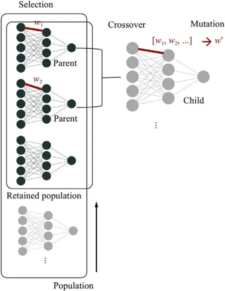
Fig. 2. Schematic of neuroevolution.The process include selection,crossover,and mutation.

Before discussing neuroevolution,we review the basics of the Jacobi method and the recent applications of machine learning in scientific computing.

First,we review the Jacobi iterative method and the recent developments.Consider a linear systemAijujbi.The Jacobi method with relaxation reads:

whereωis the relaxation factor and can potentially depend onn(time) andi(space).The Jacobi method is embarrassingly parallel,i.e.,u(n+1)depends only onu(n),but because of its slow convergence [10],its use in today’s scientific computing is not common.Yang and Mittal proposed scheduled relaxation of the Jacobi method (SRJ) [11],which accelerates the Jacobi method by a factor of 100.Their strategy is to pickPdistinct relaxation factors,ω1,ω2,...,and apply the picked relaxation factorsm1,m2,...,times in a cyclical manner.The use of different relaxation factors dates back to Refs.[12,13],but Ref.[11] gives the optimal combination of under-and over-relaxations through the following algebraic equations

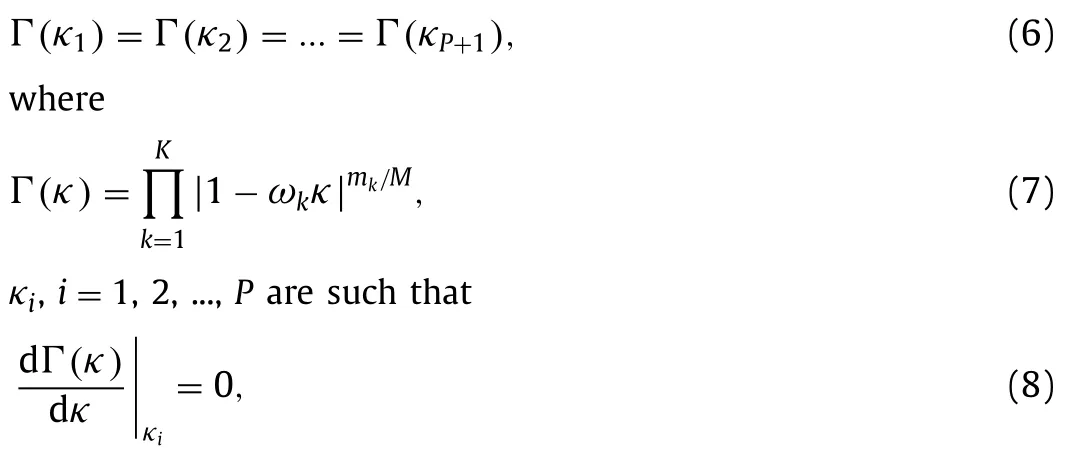
Mis the size of a iterative cycle,and 0<κ≤2 depends on the dimension of the problem,the grid size,and the boundary condition.The above equations are increasingly stiff with highPvalues.Yang and Mittal solved forK≤5.Later,Adsuara et al.[14] and Babu [15] were able to solve forKup to 15.These recent developments,including the ones in Refs.[16–19],make the Jacobi method a competitive method in parallel computing,where the increase of processor count puts a premium on parallelizability and scalability of numerical algorithms.Following this line of research,we will adapt the Jacobi method for Poisson’s equation with density discontinuities.

Next,we review applications of machine learning in scientific computing.There have been many applications of machine learning in fluid research,see,e.g.,Refs.[20–28].Its use in scientific computing is usually in a standalone manner.That is,a machine learning model directly relates inputs and outputs without being attached to any conventional iterative method [29–31].This standalone approach has led to efficient surrogate models but has limitations that prevent its use for complex real-world engineering problems.We take the recent work by Zhu et al.[29] as an example,where the authors also considered Poisson’s equation.In Ref.[29],a physics-constrained deep-learning model is developed that directly gives a solution for the Poisson equation.The model is more efficient than any conventional iterative method,but the application of this model is,at present,limited to two-dimensional problems,uniform grids,and continuous density fields.While limitations of standalone machine learning models will eventually be addressed,it is probably safe to say that,in the foreseeable future,CFD practitioners will still rely on conventional iterative solvers for real-world engineering problems.Hence,applying modern machine learning tools to solve difficulties in conventional iterative methods would be a worthwhile effort.A notable work along this line is by Islam and Wang [19].In Ref.[19],the authors trained an algorithm to select numerical schemes.The training uses convergence data obtained from randomly applying scheduled relaxation of Jacobi to a 1D Poisson problem.

In this work,we resort to neuroevolution,or evolutionary neural network (ENN).First,we explain what neuroevolution is.ENN,or neuroevolution,is a form of artificial intelligence (AI) that uses evolutionary algorithms to generate artificial neural networks(ANN),parameters,topology,and rules [32,33].It sees many applications in artificial life,game playing,and evolutionary robotics[34],but there has not been much,if any,use of this tool in the development of numerical schemes.Figure 2 is a schematic of neuroevolution.The process begins with selection:a group of ANNs is ranked according to a fitness function,which evaluates an ANN’s performance at a given task.In this work,the fitness function evaluates the convergence rate of a numerical strategy.The topranked ANNs,e.g.,the top 50%,are retained,and the rest are discarded.While keeping a couple of the non-top ANNs is benefitial in some applications [35],we see no benefit here.The next step is crossover.A pair of ANNs are used to generate a new network.The pair of ANNs are called parent networks,and the generated new network is called a child network.The child network inherits genes,i.e.,weights,biases,neural network architectures,from the two parent ANNs.For example,the weight of a particular connection in the child network isw1,w2,2w1 −w2,or 2w2−w1,wherew1andw2are the weights in the parent ANNs.The crossover step generates enough children to keep the population size unchanged.The last step is mutation:a weight in a child ANN changes.Here,the mutation strategy is to sample a number from −ctocand add that number to the weight.The network size is kept unchanged.The above three steps are repeated until we get a well-performing neural network.The reader is directed to Ref.[35] for further details of ENN.

Having reviewed the basics of neuroevolution,second,we validate the methodology by determining relaxation factors for the SRJ schemes in Ref.[11].Without loss of generality,we consider the Poisson equation on a 1D domain [11].We also assume that the density is constant and that the domain size is 1.The amplification factor of one Jacobi iteration reads

whereNis the number of grids,and the wavenumberkxis an integer from 1 toN/2.The SRJ method cycles throughMJacobi iterations and the effective amplification factor of an SRJ cycle is

whereaeffis the effective amplification factor andakis the amplification factor of thekth iteration.The grid sizeNaffectsκ’s minimum value.aeff,makis the effective amplification factor of the firstmiterations.We inputaeff,mto an ANN and let the ANN output the relaxation factor for the (m+1)th iteration,as sketched in Fig.3.We then score an ANN based on the convergence rate of the resulting SRJ cycle,i.e.,s1 −We cut off a negative score at 0.Obviously,a large score corresponds to fast convergence.We will see if neuroevolution is able to“learn”the SRJ schemes in Ref.[11].

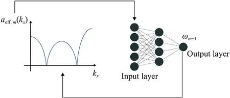
Fig.3. Schematic of how an ANN generates an SRJ scheme.

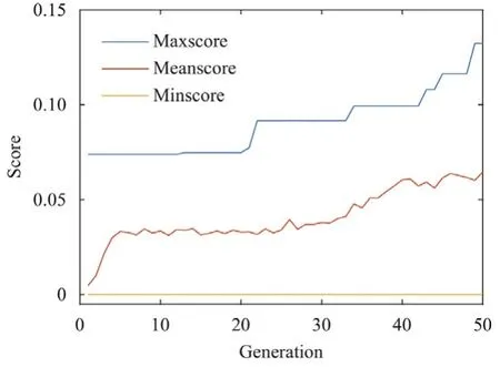
Fig. 4. Convergence history of an ENN.Here,the population size is 1000,the mutation strength c50.The grid size is N 16.

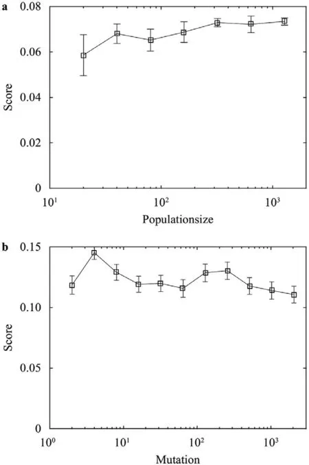
Fig. 5. a The best scored ANN after 50 generations as a function of the population size.The mutation strength c is kept constant and is 50.b The best scored ANN after 50 generations as a function of mutation strength.The population size is kept constant and is 1000.Each data point in a, b is an average of 50 trainings,and the error bars are the root-mean-square of the 50 trainings.The grid size is N 16.

For validation purposes,we constrain the number of iterations to 2.This corresponds to theM2 schemes in Ref.[11].According to Ref.[11],the two relaxation factorsω1 andω2 are solutions to the following set of algebraic equations

whereκmin2sin2(π/N).The solutions of the above equations are tabulated in Table 1 forN16 toN1024 for reference.We train ENN forN16 to 1024.Obviously,the neural networks do not“know”Eq.(11).The training halts if the best score stays constant for more than 20 generations.The best-scored ANN outputs two relaxation factors for the two Jacobi iterations.Figure 4 shows the typical convergence history of an ENN (for the first 50 generations).The best score is an increasing function,although it stays constant for a few generations from time to time.The worst score stays 0,and the average score increases gradually.We tabulate the ENNgenerated relaxation factors in Table 1.We see that the ENN and Eq.(11) lead to almost the same result.Employing the same strategy but constraining the number of distinct relaxation factors to 3 and 4,we are able to get SRJ schemes that correspond toP2(notM2) andP3 schemes (not shown for brevity).

Table 1 Relaxation factors obtained from solving Eq.(11) (the number on the left) and from ENN (the number on the right).

Before applying neuroevolution to the Jacobi iterative method for Poisson’s equation with density discontinuities,we discuss the effects of different hyperparameters.Figure 5a shows the score after 50 generations for population sizes from 20 to 1500 when the ENN is trained forP2 schemes.Figure 5b shows the score after 50 generations for mutation strengthcfrom 2 to 2000 when ENN is trained forP3 schemes.Each data point in Fig.5a and 5b is an average of 50 trainings,and the error bars are the rootmean-square of the 50 trainings.From Fig.5a,we conclude that a large population leads to a high learning rate at the cost of additional computation.From Fig.5b,we conclude that,on the one hand,a low mutation rate limits the range an ENN searches,which slows down the convergence;on the other hand,a high mutation rate makes the search unfocused,which also slows down the convergence.The effects of both the population size and the mutation rate are very much the same when training for Poisson’s equation with variable coefficients,and the results will not be shown for brevity.

Having validated our methodology,we now apply neuroevolution to adapt the Jacobi method for Poisson’s equation with density discontinuities.The strategy is to vary the relaxation factor as a function of the local density field such that the solution converges quickly.Here,we require the regular,slightly under-relaxed Jacobi iteration be applied when the local density has no gradient.With this constraint,any acceleration will be a result of our treatment at density discontinuities.An ANN will giveMrelaxation factors to be used in a cyclic manner at all locations.The resulting scheme will be applied to a 2D problem with the density field shown in Fig.6a.Our implementation of the Jacobi method is based on an alternating direction method.At the boundary across which the density is discontinuous,derivatives are evaluated parallel and normal to that boundary.With this implementation,density discontinuities are only present in the normal direction.For the particular density field in Fig.6a,the otherwise most slowly converging mode,i.e.,thekxπ/Nπ/Nmode,survives,which sets the upper bound of the convergence rate to that of Jacobi method on the same domain with no density discontinuities.Further acceleration can be achieved with treatment at locations where the density is continuous,which falls out of the scope of this discussion.We will not train the ANNs for grid size nor problem dimension.The understanding is that density discontinuities are local issues,in the sense that if a strategy handles density discontinuities for a grid and a dimension (e.g.,2D),it should work for other grids and other dimensions (1D,2D,3D,...).

Figure 7 is a sketch of an ANN in the population.The ANN has three layers.The hidden layer contains from 5 to 10 neurons.Its input is the local density field,and its output is a set of relaxation factors.The ANN is constrained such that it givesω0.99(slightly under relaxed) if the density field is continuous.The ANNs are trained on a 2D grid of sizeN64 for the density field as shown in Fig.6a.Each training takes about two hours on a laptop.The most costly part is the evaluation of the resulting schemes of an ENN population.In the following,we summarize the results.Again,slightly under-relaxed Jacobi is applied at locations where the density is continuous,and we vary the relaxation factor at locations where the density is discontinuous by cyclically applyingMrelaxation factors.We refer to the resulting scheme as JacEM.Figure 8 shows the convergence rate of JacE8,JacE16,and JacE32 forr0.001.A large cycle allows for more degrees of freedom and therefore leads to better-performed schemes.For JacE32,the convergence rate is already the same as the Jacobi scheme on a constant density field.Figure 9a-9c shows the asymptotic convergence rate of JacE16 forr0.001,r0.01,andr0.1,respectively.Comparing the thin black lines in Fig.9a-9c,which represent the asymptotic convergence rate of the regular Jacobi scheme,we see that the density discontinuities become less challenging as the strength of the density discontinuity decreases.As a result,having 16 iterations in a cycle already allows the resulting scheme to converge as fast as the Jacobi scheme on a constant density field forr0.01 andr0.1.

Fig.6. Density field of a a 2D field with discontinuities, b a 1D field with discontinuities,and c a 3D field with discontinuities.The field in a is the field we train for.Here,r is the strength of the density discontinuity.The low density region spans two grid points in the vertical direction.

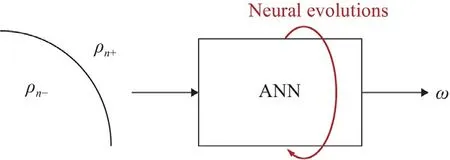
Fig. 7. Sketch of an ANN.Its input is the local density.Its output is a set of relaxation factors to be used at the location.

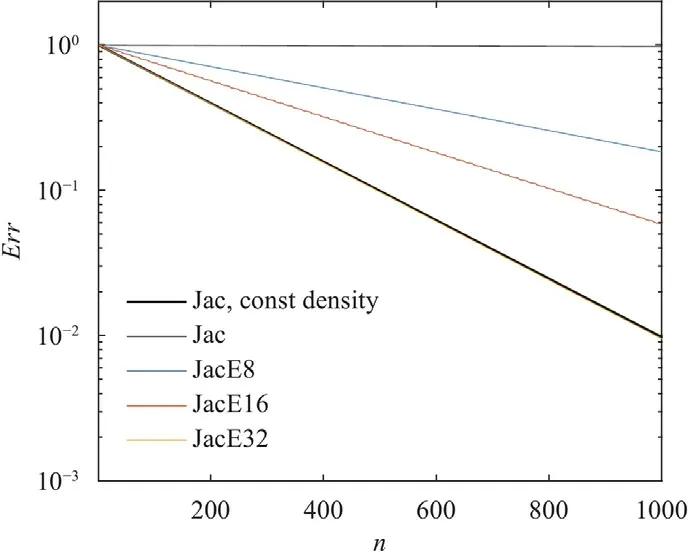
Fig. 8. Convergence history of the Jacobi method (thin black line),JacE8,JacE16,and JacE32.JacEX contains X Jacobi iterations.The density field is shown in Fig.6a with the strength of density discontinuity r being 0.001.The convergence history of the Jacobi method on a constant density field is also shown for comparison.

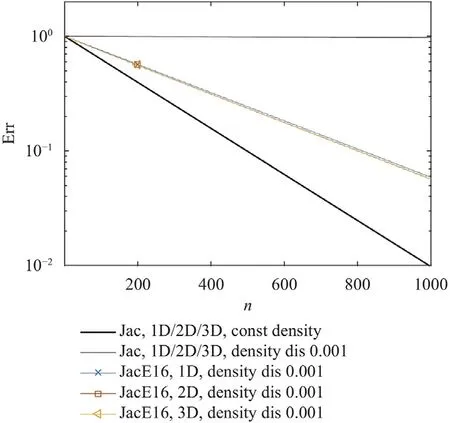
We have previously argued that we only need to train ANN on a single,2D grid for the resulting scheme to be applied on any grid in any dimensional space.In the following,we present some supporting evidence.Figure 10a-10c show the asymptotic convergence rate of the JacE16 scheme on 2D grids of size 32×32,64×64,and 128×128,respectively.The convergence rate of a Jacobi scheme scales as ∼1/N2[9].For presentation purposes,we have adjusted the range of theyaxis such that the Jacobi scheme applied on a constant density field yields the same slope.We see that density discontinuity remains an issue irrespective of the grid size,which is consistent with the results in Fig.1.We also see that JacE16,trained on a grid of sizeN64,provides a similar level of acceleration on grids whose sizes areN32 andN128.Last,Fig.11 shows the asymptotic convergence rate of JacE16 on the one dimensional and three dimensional grids shown in Fig.6b and 6c.Again,the same scheme,JacE16,gives very similar acceleration on 1D and 3D grids as on a 2D grid.

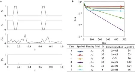
Fig.1. a Density fields.ρI represents the density field of liquid bubbles in a gaseous environment.ρII represents the density field of gaseous bubbles in a liquid environment.ρIII is a random density field.ρIV ≡1 is a constant density field.b Convergence history.The residual is normalized by the initial residual (i.e.,the residual at iteration 0).The legend is tabulated in the table. N is the grid size. n10 is the number of iterations needed to reduce the residual by a factor of 10 (asymptotically).“Jacobi”refers to the Jacobi iterative method,and“G-S”refers to the Gauss-Seidel iterative method.

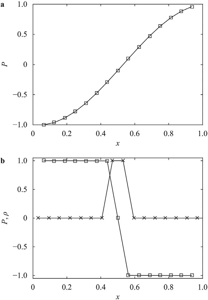
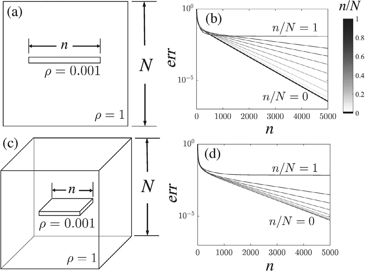
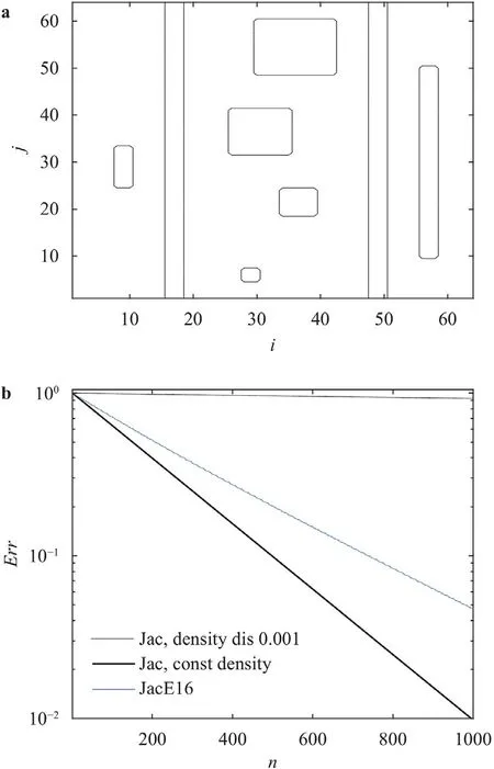
The discussion so far has focused on quasi-one-dimensional problems.While many problems are more challenging with threedimensional features [36,37],the numerical issue due to density discontinuities is the opposite.To show that,we solve the Poisson equation on the density fields in Fig.12a and 12c,where a thin layer of fluid with densityρ0.001 lies in a fluid of densityρ1.The domain size isN32.The problems are quasi one dimensional ifn/N1,and two-dimensional/three-dimensional if 0

Fig. 10. Convergence history of the JacE16 scheme on a a mesh of size 32×32,b a mesh of size 64×64,and c a mesh of size 128×128.The distribution of the density discontinuities is shown in Fig.6a.

Fig. 11. Convergence history of the JacE16 scheme on one dimensional,two dimensional,and three dimensional grids.The convergence rate of the regular Jacobi scheme on a constant density field does not depend on the problem’s dimension.The same is true for the regular Jacobi scheme applied to problems with density discontinuities.Here,“density dis”is short for density“discontinuity”.

From a practical standpoint,applying ENN addresses the issue due to discontinuities in the density field.However,relying on AI,which is a black box,gives little physical understanding.In the following,we will try to understand how neuroevolution solves the problem by looking into the error equation,i.e.,Eq.(3).Define the asymptotic mode to be the mode that determines the convergence rate.Figure 14a and 14b show the asymptotic modes for constant and variable coefficient Poisson equation with Neuman boundary conditions,respectively.The Jacobi scheme reads forρConst.Per Eq.(12),information from the right cell ati+1 and the left cell ati−1 have equal rights on the center cell ati.

Fig.9. Convergence history of JacE16 for a r0.001, b r0.01,and c r0.1.

The Jacobi scheme reads

leading to the asymptotic mode in Fig.14b.To help information get fromρ1 toρ0.001,we should assign a high weight for the solution at theρ1.Bearing that in mind,we now look at the Jacobi scheme with over relaxation:

Fig. 14. a Asymptotic mode for constant coefficient Poisson equation.A Neumann boundary condition is applied at the two ends of the domain.b Density (× symbols) and the asymptotic mode (☐symbols).

Invoking Eqs.(14) and (15) leads to

Fig.12. a Density field.A thin layer of fluid of density ρ 0.001 is placed in a fluid of density ρ 1.The grid size is N 32.The thin layer spans two grids. b Convergence history.The pressure field is solved for the density field in a. n/N 0 corresponds to a constant density field. n/N 1 corresponds to a quasi-one-dimensional density field.The lines are color-coded. c Density field.The thin layer spans two grids. d Convergence history.The pressure field is solved for the density field in c.

Fig.13. a Density field.The density discontinuity is r 0.001. b Convergence of the JacE16 scheme on the density field in a.We show the convergence of the regular Jacobi method on the density field in a and that of the regular Jacobi method on a constant density field for comparison.

Ifω500.5,Eq.(16) reduces to Eq.(12),which equally weights information fromPi+1andPi−1.Hence,a large relaxation factor would help address the slow convergence of the Jacobi method for the pressure Poisson equation with density discontinuity,which is consistent with our ENN.JacE8 atr0.001 has a large relaxation factor around 950 and 15 small relaxation factors around 0.51.JacE16 atr0.001 has a large relaxation factor around 3500 and 15 small relaxation factors around 0.51.The above analysis is,however,not rigorous.Applyingω500.5 at density discontinuities is numerically unstable (not shown for brevity),which is why we had resorted to machine learning in the first place.In general,attempting to interpret results of an artificial neural network is hard and dangerous [38],and here we will refrain from more in-depth analysis.

Last,we summarize.In this letter,we apply neuroevolution to adapt the Jacobi method for Poisson’s equation with density discontinuities.Because of a lack of known numerical strategies (labeled data),the task can not be tackled with supervised learning.This makes neuroevolution,a form of AI that requires only a measure of performance,an ideal tool.We validate the methodology by applying it to SRJ.We show that the evolutionary network is able to learn the known best strategy,yielding relaxation factors that are the same as the ones reported in the literature.After validating our methodology,we apply neuroevolution to the Jacobi method for the pressure Poisson equation with density discontinuities.We show that ENN leads to a set of relaxation factors,with which the Jacobi method efficiently handles density discontinuities for all grids.In all,this work presents a successful attempt in applying AI in the framework of conventional numerical schemes.While the discussion here is limited to the Jacobi method and the pressure Poisson equation,the framework can well be used to adapt any numerical schemes.

DeclarationofCompetingInterest

The authors declare that they have no known competing financial interests or personal relationships that could have appeared to influence the work reported in this paper.

Acknowledgements

The authors hope to thank Ting Zhou for her help in developing our Python code.Yang thanks Robert Kunz for fruitful discussion.Yang acknowledges ACI and XSEDE for CPU hours.Shi acknowledges financial support from the National Natural Science Foundation of China (Grant 91752202).