Computing mean fields with known Reynolds stresses at steady state

Xinwen Guo ,Zhenhu Xi ,Shiyi Chen c,

a State Key Laboratory for Turbulence and Complex Systems, College of Engineering, Peking University, Beijing 100871, China

b Department of Engineering Mechanics, Zhejiang University, Hangzhou 310027, China

c Department of Mechanics and Aerospace Engineering, Southern University of Science and Technology, Shenzhen 518055, China

Key words:RANS Propagation error Nonlinear Reynolds stresses

ABSTRACT With the rising of modern data science,data-driven turbulence modeling with the aid of machine learning algorithms is becoming a new promising field.Many approaches are able to achieve better Reynolds stress prediction,with much lower modeling error (∊M),than traditional Reynolds-averaged Navier-Stokes(RANS) models,but they still suffer from numerical error and stability issues when the mean velocity fields are estimated by solving RANS equations with the predicted Reynolds stresses.This fact illustrates that the error of solving the RANS equations (∊P) is also very important for a RANS simulation.In the present work,the error ∊P is studied separately by using the Reynolds stresses obtained from direct numerical simulation (DNS)/highly resolved large-eddy simulation to minimize the modeling error ∊M,and the sources of ∊P are derived mathematically.For the implementations with known Reynolds stresses solely,we suggest to run an auxiliary RANS simulation to make a first guess on ν∗t and S 0ij .With around 10 iterations,the error of the streamwise velocity component could be reduced by about one-order of magnitude in flow over periodic hills.The present work is not to develop a new RANS model,but to clarify the facts that obtaining mean field with known Reynolds stresses is nontrivial and that the nonlinear part of the Reynolds stresses is very important in flow problems with separations.The proposed approach to reduce ∊P may be very useful for the a posteriori applications of the data-driven turbulence models.

Turbulence is ubiquitous in nature and engineering applications[1] and it is one of the main research topics in fluid mechanics.Thanks to the rapidly development in computer technology and the numerical algorithms,numerical simulation is becoming a more and more important tool to study turbulence.Although direct numerical simulation (DNS) and large-eddy simulation (LES) can obtain more accurate predictions on turbulence,Reynolds-averaged Navier-Stokes (RANS) is still the most popular simulation approach in engineering design and applications.In RANS simulations,extra unclosed terms,known as the Reynolds stresses,arise due to the nonlinearity of the convective term in the momentum equations,and thus some treatment,the RANS modeling,should be adopted to close them [2-4] .

Let’s take the incompressible flow as an example,where the governing equations are as follows:

HereRij〈uiuj〉 is the unclosed Reynolds stress tensor withUi〈Vi〉 anduiVi−Uibeing the Reynolds averaged flow field and the corresponding fluctuations of the instantaneous fieldVi.Thanks to the continuous effort by the turbulence community,many different types of models have been proposed for RANS simulations [5–7],either with the Boussinesq eddy-viscosity approximation (Algebraic models or zero-equation models [8],one-equation models [9] and two equation models [10–12]) or beyond it (stresstransport models [ 13,14 ] and nonlinear models [15]).As sketched in Fig.1,two different types of errors could exist for a typical RANS simulation.One is the model error∊M,which comes out whenRijis estimated through the RANS models and it can be denoted as∊Mwithandbeing the true Reynolds stresses and the modelled Reynolds stresses respectively.The other is the propagation error∊P,which appears when the RANS governing Eqs.(1) and (2) are solved with RANS closure models inserted.In the past,when a RANS model is evaluated inaposterioritests,the final numerically solved mean fieldswill be compared to the reference true valuesand the deviation will be referred as the error of the RANS model and it was commonly used as the criterion to evaluate the performance of the RANS model.In fact,the above deviation can be separated into two parts,i.e.

In fact,solving the RANS governing Eqs.(1) and (2) with RANS closure models inserted is nontrivial,especially when a RANS model beyond the Boussinesq eddy-viscosity approximation is considered.At some situations,it is even difficult to obtain a convergent solution [16,17],making∊Pan important issue that needs to be treated seriously.This is especially true for the applications of the data-driven turbulence models [18-27].For most of data-driven RANS models,no explicit expression for the Reynolds stress tensor can be obtained [20,22,23],and the numerical instability issue is even severer and∊Pcould be very large.In Ref.[22],they reported that the mean velocity field obtained with their data-driven RANS model does not match better with the DNS data than the original RANS model,even though their RANS model can predict better Reynolds stresses.In Ref.[16],they believed that RANS equations with explicit data-driven RANS models can be ill-conditioned.This ill-conditioning problem is more complicated than a numerical issue which can be resolved by changing different discretization schemes or other specific numerical tricks (It should be noted that Yin et al.[28] reported a less severe ill-conditioning problem for flow over periodic hills when a compressible solver was used).Even for the channel flow,which is a simple case with vanishing convective terms,the ill-conditioning problem still exists and gets more severe with increasing Reynolds number [16].In order to make the RANS simulations more stable,they proposed an implicit treatment.With the information of the strain-rate tensor from the DNS database,this implicit treatment can also reduce∊Pto a very low level.Nevertheless,the consistent and accurate strain-rate tensor is not always known in advance,which limits the usage of this implicit treatment.

On the other hand,it has been shown by Thompson et al.[29] that the error of solving RANS equations with Reynolds stresses from accurate DNS can still be very large.With friction Reynolds numberReτ5200 in turbulent channel flow,a 0.41%maximum error in turbulent shear stresses could finally lead to a 21.6% volume-averaged error in the mean velocities [16,29].In Ref.[30],Poroseva et al.confirmed that the errors resulting from insufficient sample size in DNS are very important for the RANSDNS simulations to obtain accurate turbulent statistics,although all terms but the molecular diffusion in the RANS equations were represented by the data from DNS.In Ref.[20],they also reported that their predicted streamwise velocity using true DNS anisotropy behaves differently from the true DNS Fig.5 in Ref.[20]).From these results,we may conclude that∊Pcould be very large if the RANS governing Eqs.(1) and (2) are not solved in a numerically stable and converged way.

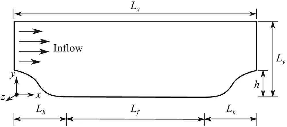
Fig. 2. Sketch of computational domain for flow over 2D periodic hills.The hill height is denoted by h.The total length and height of the whole domain are denoted by L x and L y respectively.

The present paper aims to study the propagation error∊P,i.e.to quantify the errors of the mean flow fields when they are solved with known Reynolds stresses.In order to minimize the influence of∊M,the Reynolds stresses obtained from DNS or highly resolved LES are adopted.Different from the previous work in Ref.[16],we consider the situation where the only known information is the Reynolds stresses from DNS or LES.We will derive the source of∊Pand propose two possible algorithms to reduce it.It should be noted that we are not proposing a new RANS model,but clarifying the fact that∊Pis inevitable in real applications.The proposed algorithms indeed can reduce∊Pto a relative low level and they might be useful for theaposterioriapplications of the data-driven turbulence models.Furthermore,our numerical results also show that the nonlinear part of the Reynolds stresses is very important in flow problems with separations.

Firstly,we would like to review the implicit treatment with known true values of Reynolds stresses and mean strain rateandfrom Wu et al.[16].Here,the true values could be obtained from DNS or highly resolved LES.Considering the momentum equation appeared in Eq.(2) at steady state,with the deviatoric anisotropic part of Reynolds stress tensoraij〈uiuj〉−2kδij/3 and an alternative pressurep/ρ+2k/3,the momentum equation can be rewritten as

for incompressible flows.Here,

is the nonlinear part of the Reynolds stresses,is the discrete mean strain rate tensor from the DNS or highly resolved LES field withδ/δxjbeing the difference operator whose exact form shall depend on the numerical scheme and mesh information,νtis the turbulent eddyviscosity,which is the key to quantify and balance the amount of Reynolds stresses to be treated implicitly.It should be noted thatνtcannot be zero.Otherwise,the implicit treatment will be degraded to the explicit treatment which will suffer from the ill-conditioning problem.With the above decomposition Eq.(5),Wu et al.[16] found that it is easier to obtain a stable discrete solutionwith some algorithms (such as SIMPLE algorithm)and the discrete solutionsatisfies the following difference equation

Here,erris the residual error during the iterations.

Equivalently,the above Eq.(7) can be reformed as

being the main source of∊P.Here,is the discrete mean strain rate tensor from the discrete solutionIdeally,if converged solutionis obtained and it approaches to∊Pcould be eliminated.However,the inconsistence betweenanddue to the inaccuracies of the DNS or highly resolved LES data [30] as well as the existence oferrmakes∊Pinevitable.Different choices ofνtwill result in differentEP and∊Paccording to Eq.(9).A proper choice ofνtmay reduce∊Pto a relatively low level,andνtwas chosen to be the optimal eddy viscosityby Wu et al.[16] as

Now,we are considering a different situation,that is the propagation with knownand unknownWe want to answer one question:can we get a good prediction on the mean field when we only know the correct Reynolds stressesThis is a fundamental question for steady RANS simulations and it is closely related to the data-driven RANS models without explicit expressions.

Similar to the decomposition in Eq.(5),can still be decomposed with any other knownandas

being the source of∊Pat then-th iteration step.The final∊Pwill be determined by allin the pastniteration steps,accumulatively,and thus bothandare very important.From the above derivation,∊Pseems inevitable unless the accumulative effect ofin the pastniteration steps could cancel with each other coincidentally,which is a virtual impossibility.Therefore,we may arrive at the following conclusion that even though a correct prediction on the Reynolds stresses could be obtained,one may still be unable to compute the mean field accurately if only the information on the Reynolds stresses is known.

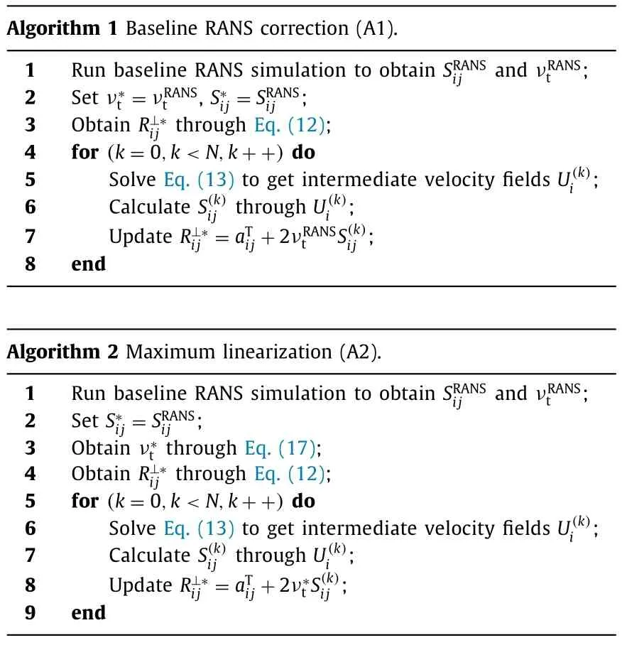
In the following,the above two choices will be denoted as algorithm A1 and A2 respectively.Details of these two methods are summarized in Algorithms 1 and 2.

In Wu et al.[16],they showed that they could obtain the mean field with a relatively low error using their implicit treatment in flow over two-dimensional (2D) periodic hills with knownandat Reynolds numberReUh/ν5600.Here,his the hill height,Uis the bulk velocity at inflow section andνis the kinematic viscosity.In this section,we are going to numerically study what kind of mean velocity field can be obtained if we only knowThe same flow problem as Wu et al.[16],the flow over 2D periodic hills,is chosen as the test case.Due to its relatively simple geometry and well-defined boundary conditions [31-34],it has often been used as a benchmark test case for modeling and simulation issues,such as subgrid-scale models and wall functions in LES[32,35,36],data-driven turbulence modelings [22,23,37].A sketch of the basic geometry is shown in Fig.2.The streamwise and vertical directions are denoted asxandyrespectively.The hill length is denoted byLhand the length of flat part of bottom wall is denoted byLf.An accurate specification for hill shape is available in form of piece-wise polynomials in Refs.[31,34].

A 2D structured grid is adopted with resolution 128 × 160 in streamwise and normal directions.The grid is refined in the near wall region to ensure that the height of the first cell center above the wall in wall unit is less than one for all cases and the grid independence has been checked.The RANS grid used here is coarser than the fine DNS or highly resolved LES grid,and the error could exist when the data are interpolated from the fine DNS or highly resolved LES grid to the coarse RANS grid using the nearest points.However,we are using the same RANS grid and the same interpolated Reynolds stresses in our studies,which can minimize the influence of this source of error.All RANS simulations are conducted via the steady-state solver "simpleFoam" based on SIMPLE algorithm (for semi-implicit method for pressure-linked equations)[38] from the widely used open-source platform OpenFOAM [39].For the numerical discretizations,the second-order central difference scheme is adopted for all terms except for the convection term,which a second-order upwind scheme is used.Please note that we are not specifying a detailed RANS model here and any RANS model with corresponding eddy viscosity can be used.The detailed information on RANS models will be specified when they are used.The flow is set to be periodic in the streamwise direction.No-slip condition and zero-gradient condition are set at walls for velocity field and pressure respectively.

As the first test,we would like to show the results of the two algorithms atRe10,595 with the Spalart-Allmaras (SA) model[9] as the auxiliary RANS model.The Reynolds stresses and reference mean field data are from Breuer et al.using the highly resolved LES [33].The ratioσ≡is used to quantify the error of solved mean velocity fieldUjto the reference mean velocity fieldwhereδUrms andare defined as [16]

Here,[φ]jdenotes thej-th component of theN-vector obtained by discretizing the fieldφ(φU,UTor other variables) on theNx×Nymesh withNNx×Ny,ΔVjstands for the volume of thej-th cell andVis the total cell volume in the domain.

Figure 3 shows the errors of streamwise and vertical mean velocities forRe10,595 with SA model as the auxiliary RANS model via two algorithms as the iteration advances.It is seen that the errors of two velocity components from algorithm A1 and A2 generally decrease with the iteration.They decay very fast during the first two iterations and then become slowly if the iteration goes on.The errors from algorithm A1 are lower than those from algorithm A2.ForUxandUy,σare about 0.018 and 0.078 for algorithm A1 while they are about 0.031 and 0.120 for algorithm A2 after 10 iterations.Comparing to the corresponding errors from the propagation with knownwhich are 0.0083 and 0.042,the errors for algorithm A1 are about twice while those for algorithm A2 are about four or three times.Considering that algorithm A1 and A2 do not need the information aboutthe increases of errors are acceptable.Furthermore,the errors from baseline RANS simulation (see the errors at the zeroth iteration step in Fig.3),which are about 0.113 and 0.412,are one order of magnitude larger than those with the correct Reynolds stresses.In order to further show the differences among different results,the mean streamwise velocity profiles from two different algorithms,as well as those from the reference values and the baseline RANS simulation,at 9 different locations are shown in Fig.4.

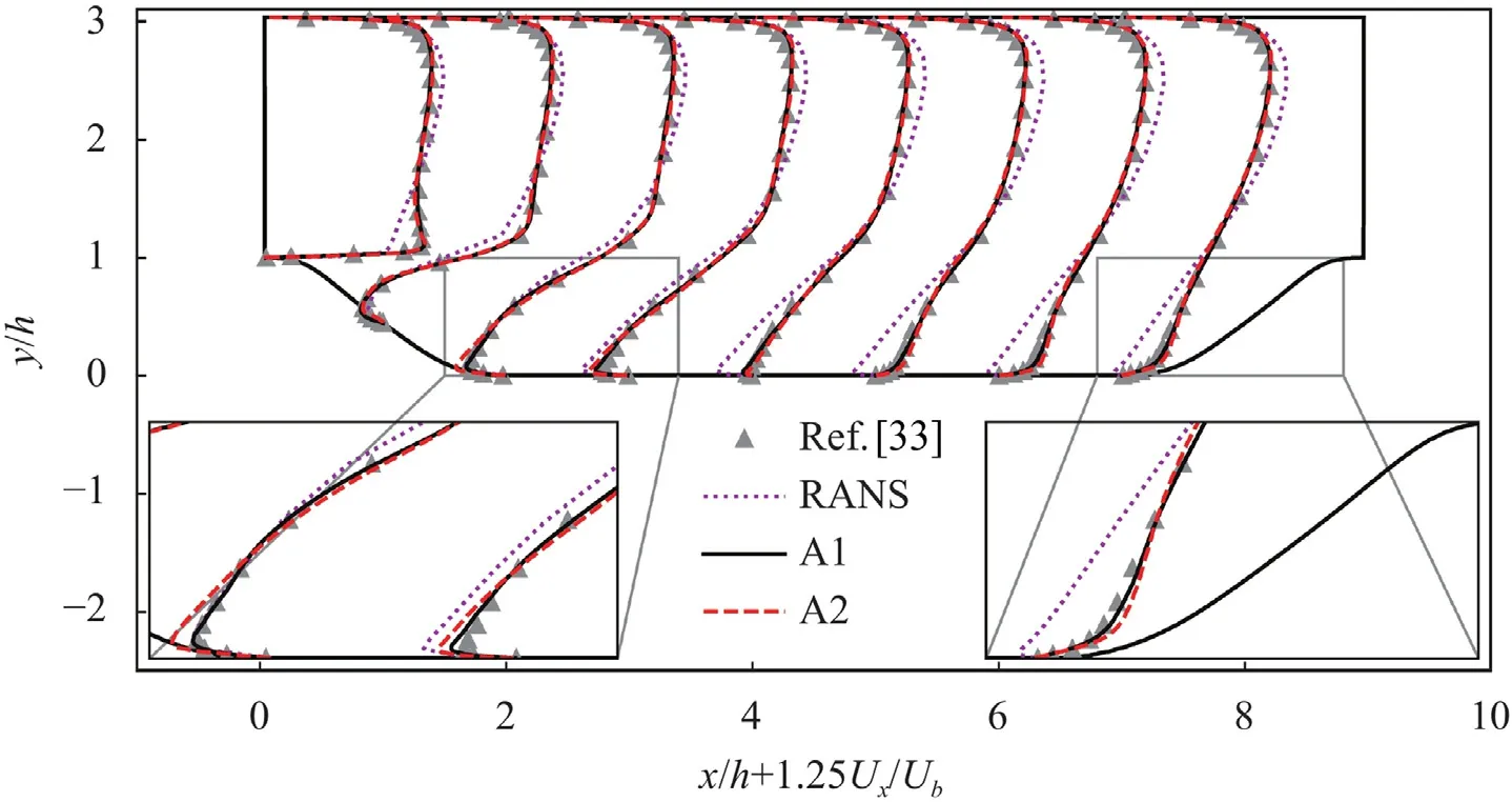
Fig.4. Propagated streamwise mean velocity profiles at 9 separated locations from Re10,595 from the algorithms A1 and A2.The highly resolved LES data (Ref.[44]) and RANS-SA results are also shown for comparison.

Firstly,it is seen that the baseline RANS with SA model fails to predict the mean velocity profiles at 9 locations as compared to the reference profiles from the highly resolved LES.Fictitious backflows can still be observed even atx/h6 for RANS-SA simulation.It is interesting to note that although the baseline RANS predict the mean velocity very poorly,it still can help to promote the prediction of the algorithm A1 and A2 as shown in Fig.4,where the mean streamwise velocity profiles at 9 different locations match very well with the reference data.Compared to the baseline RANS simulations,the algorithm A1 has the same eddy viscosity besides the additional nonlinear Reynolds stresses.The better prediction on the mean velocities of the algorithm A1 over the baseline RANS then well documents the importance of the nonlinear part of the Reynolds stresses in this kind of flow problems with separations and reattachments.It should be noted that a comparison between a nonlinear RANS model and a linear RANS model might also be used to show the importance of the nonlinear part of the Reynolds stresses.However,the modeling error might complicate the comparison,and we cannot guarantee that the results from the nonlinear RANS model are better than those from the linear RANS model.In the present work,by using the accurate Reynolds stresses from the highly resolved LES,the influence of the modeling error is minimized and the algorithm A1 can get better results than the baseline RANS simulations (see the data at the zeroth iteration step in Fig.5 below),which can clearly show the importance of the nonlinear part of the Reynolds stresses.The algorithm A2 also can get a very good prediction on the mean velocity profiles,although a little poorer than the algorithm A1.These results then illustrate that the choice ofνtwill influence the final results to a certain degree.

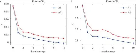
Fig.3. Errors of propagated velocity for Re10,595 at different iteration steps with SA model as the auxiliary RANS model via algorithms A1 and A2: a streamwise velocity U x and b vertical velocity U y.The corresponding errors for U x and U y using known are about 0.0083 and 0.042 respectively.

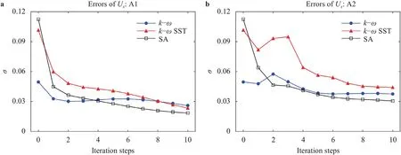
Fig.5. Errors of propagated velocity U x using A1 a and A2 b with different auxiliary RANS models at Re10,595.

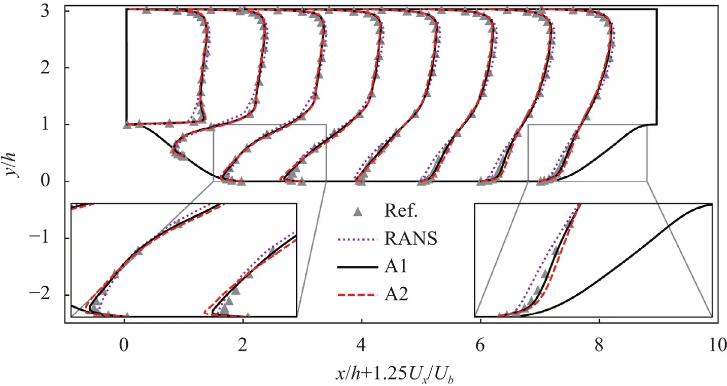
Fig. 6. Propagated streamwise mean velocity profiles at 9 separated locations for Re10,595 from the algorithms A1 and A2 with k-ω model being the auxiliary RANS models.

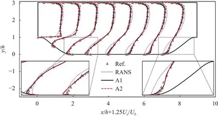
Fig.7. Propagated streamwise mean velocity profiles at 9 separated locations for Re10,595 from the algorithms A1 and A2 with k-ω SST model being the auxiliary RANS models.

Since the choice ofνtwill affect the final results,the different choice of auxiliary RANS models will surely affect the final results.Fig.5 shows the errors ofUxusing A1 and A2 with three different auxiliary RANS models,including the SA model,thek-ωmodel[6] and thek-ωshear stress transport (SST) model [40].It is seen that both algorithms A1 and A2 can effectively reduce the errors to a relatively lower level,as compared to the errors of baseline RANS simulations,i.e.the errors at the zeroth iteration,although they are different for different models.Clearly,A1 is more stable than A2 and its errors are also smaller,again confirming that A1 is better than A2.This might be due to the different choices ofνtin A1 and A2.In A1,it is from the auxiliary RANS model and it is generally continuous and smooth in the field.In A2,νtis obtained through Eq.(17),and there might be some local extremum values andνtmight not be as smooth as that in A1,causing some potential numerical instabilities and affecting the final results.Figures 6 and 7 show the propagated streamwise velocity profiles at 9 separated locations forRe10,595 from the algorithm A1 and A2 with thek-ωand thek-ωSST model being the auxiliary model respectively.For thek-ωmodel shown in Fig.6,although it can work very well for this problem (see the errors at the zeroth iteration step in Fig.5),the algorithms A1 and A2 with the accurate Reynolds stresses from the highly resolved LES can still better predict the streamwise mean velocity profiles in most locations except the near wall results at the fourth locationx/h3 (see the zoomed-in results shown in the left-bottom corner).For thek-ωSST model shown in Fig.7,it is seen that the algorithm A1 with accurate Reynolds stresses can predict much better mean velocity profiles at all 9 locations,while the algorithm A2 can only show better predictions in the bottom region,while its results near the upper wall show clear deviations.These results again confirm that the choice ofνtmay also influence the final results,and that the algorithm A1 is superior over the algorithm A2.

The two algorithms have also been tested on different geometries and different Reynolds numbers.Here,we would like to show the results from the flow over periodic hills with a steeper hill shape atRe5600,where the hill lengthLhis shorten by a factorα0.5 whileh,LfandLyare kept the same (Hereafter,this case is denoted as "flow over steeper hills").The DNS data is from Xiao et al.[34].For this flow case,massive separation occurs and a second small circulation bubble can also be observed near the foot of the hill underneath the main big circulation bubble (see Fig.2c in Ref.[34]).Figure 8 shows the errors of propagated streamwise and vertical velocity components for flow over steeper hills atRe5600 using the algorithm A1 and A2 with the SA model being the auxiliary model.The comparisons of the corresponding streamwise mean velocity profiles at 7 separated locations are shown in Fig.9.It is seen that the errors of the streamwise and vertical velocity components can decay a lot when the iteration advances for both algorithms.The streamwise mean velocity profiles at 7 different locations also confirm the better predictions at most of the domains for the algorithm A1 and A2.

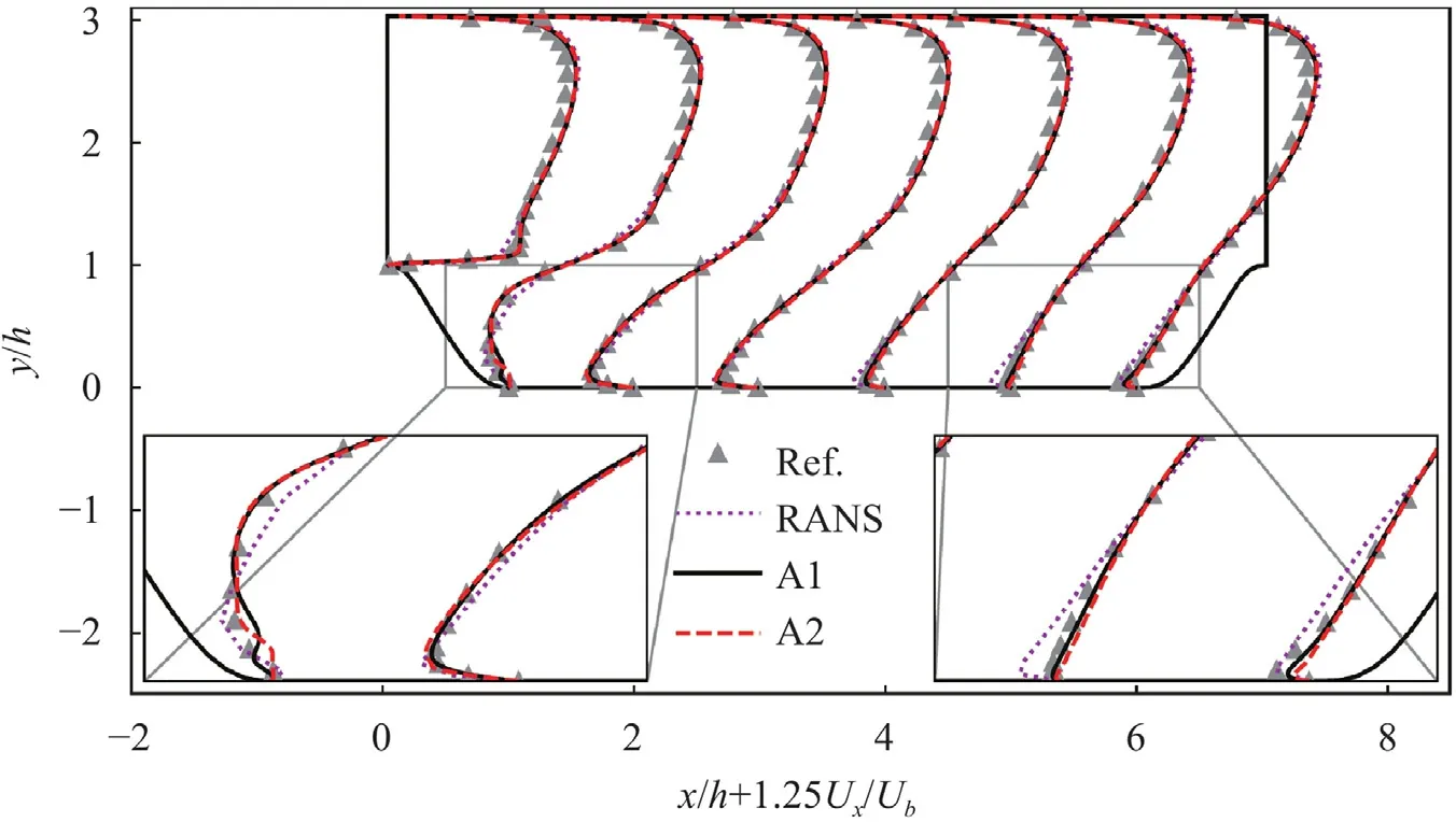
Fig.9. Propagated streamwise mean velocity profiles at 7 separated locations for flow over steeper hills from the algorithms A1 and A2.The DNS data and RANS-SA results are also shown for comparison.

In the above discussions,we have shown that settingcan generally reduce∊Pto a lower level.However,from Eqs.(14) and (15),other choices could still be adopted.For example,we could set

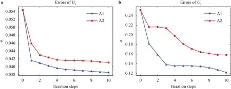
Fig.8. Errors of propagated velocity for flow over steeper hills at different iteration steps with SA model as the auxiliary RANS model via algorithms A1 and A2:a streamwise velocity U x and b vertical velocity U y.The corresponding errors for U x and U y using known are about 0.0031 and 0.058 respectively.

whereCis a constant in the whole domain,which can be constant or changing during iterations.It should be noted thatCcould be spatially varying throughout the domain.However,this could complicate the implementations since it is very difficult to determine the values ofCon each grid point in advance.With a fixed value ofC,it can be proved that a largerCcan reduce the volumeaveraged condition number and the Eq.(13) can converge much faster.However,it can be seen from Eq.(15) that a largerCmight increase the error ofFor SA model,the numerical tests show thatC≈0.7 could get a slightly better prediction on the mean velocity field.However,we could not determineCin advance without testing which surely will restrict its implementations.

Another choice is to include the history effect when estimatesat then-th step,such as or we could use the adaptive gradient algorithm [41] or "Adam"algorithm [42] to make a better estimation onHowever,based on our numerical tests,we can only lower the error a little bit.

In the above,we have showed,mathematically and numerically,that it is nontrivial to compute the mean field accurately when only the accurate Reynolds stresses are known.In fact,we may even not sure about the existence and uniqueness of the solution to such a problem mathematically,i.e.Eqs.(1) and (4) with knownaijand proper boundary conditions.In the applications of RANS simulations,Rijcould generally be obtained through some RANS models whileSijcan only be estimated from the current field.Supposing that there is some error∊Mon RANS models,i.e.,+EijwithEijbeing the deviations of the modelled Reynolds stresses to the true Reynolds stresses,then we can obtained the same expression on Eq.(14) but with a different

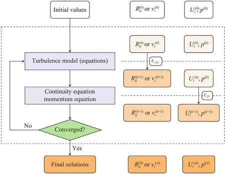
Fig.1. Overview of processes for a typical RANS solver.

In traditional RANS simulations,the propagation error∊Pof obtaining the mean fields with known Reynolds stresses was usually misinterpreted as a part of the modeling error,and has seldom been discussed alone.This makes the judgement on the turbulence models very ambiguous,especially for the data-driven turbulence models which are very popular nowadays.In the present paper,we studied the propagation error∊Psolely by using the Reynolds stresses from highly reliable DNS or LES databases,and the sources of∊Pwere derived for the situations with or without knownFor general implementations without knownthe choice ofis very critical.If it is too small,the numerical algorithm may be unstable which will increase the error due to the numerical algorithm.On the other hand,if it is too large,it will increase the iteration errors during two adjacent iterations instead.An auxiliary RANS simulation was suggested to make a first guess onand a good,stable choice is settingto the eddy viscosity from the RANS simulation.With around ten iterations,the error of mean velocity could be reduced by one-order of magnitude in the flow over the 2D periodic hills.The present work does not intend to develop a new RANS model,but to clarify the fact that obtaining the mean field with known Reynolds stresses is nontrivial.The proposed algorithms may offer some valuable references for turbulence models beyond the Boussinesq eddy-viscosity approximation to obtain satisfactory mean velocity fields.Furthermore,our work is also in favor of doing theaposterioritests for the validations when new RANS models are developed.

Another outcome of the present work is related to the modeling issue.The algorithm A1 can be viewed as a nonlinear correction to the auxiliary linear eddy-viscosity RANS model.The better prediction using A1 on the mean velocity fields over the baseline RANS model confirms the importance of non-linear part Reynolds stresses,especially for the current type of flow problems with flow separations.This information,that the nonlinear part of the Reynolds stresses is very important in separated flows,may be helpful for those groups who are trying to develop advanced datadriven RANS models.

DeclarationofCompetingInterest

No potential conflict of interest was reported by the author(s).

Acknowledgement

We would like to thank the contributions from Prof.Heng Xiao and Dr.Jinlong Wu from Virginia Tech.This work was supported by the National Natural Science Foundation of China (Grants 11822208,11988102,11772297,91852205 and 91752202) and Shenzhen Science and Technology Program (Grant KQTD20180411143441009).Xia was also supported from the Fundamental Research Funds for the Central Universities.