Why neural networks apply to scientific computing?

Shaoqiang Tang ,Yang Yang

HEDPS and LTCS, College of Engineering, Peking University, Beijing 100871, China

Keywords:Neural networks Universal approximation theorem Backpropagation algorithm

ABSTRACT In recent years,neural networks have become an increasingly powerful tool in scientific computing.The universal approximation theorem asserts that a neural network may be constructed to approximate any given continuous function at desired accuracy.The backpropagation algorithm further allows efficient optimization of the parameters in training a neural network.Powered by GPU’s,effective computations for scientific and engineering problems are thereby enabled.In addition,we show that finite element shape functions may also be approximated by neural networks.

Most scientific/engineering problems are formulated in terms of equations.The major components in an equation-based computation are function approximation and numerical scheme.The former designates finitely many entities to represent functions in a discrete manner,while the latter determines these entities by direct or recursive evaluations.For instance,piecewise constant or polynomials are adopted in finite difference and finite volume methods,whereas linear combination of shape functions is used in finite element methods.

Particularly in recent several decades,neural networks emerged as an effective paradigm in scientific and engineering explorations,succeeded first in pattern recognition,control theory and engineering,and signal processing,then expanded horizon of applications to much broader scope of scientific computations such as fluid motion detection,parameter identification,etc.[ 1,2 ].

As neural networks differ literally from most standard computational methodologies,a natural question arises:why neural networks apply to scientific computing? We see three thrusts in neural networks that contribute to the answer.First,by universal approximation theorem,deep neural networks are capable to approximate functions.Secondly,backpropagation algorithm substantially enhances the efficiency in updating undetermined parameters in a neural network.Finally,graphics processing unit (GPU) facilitates high-performance parallel implementation of the backpropagation algorithm.In this tutorial letter,we shall expose the universal approximation theorem and the backpropagation algorithm.We further introduce a neural network based on finite element shape functions.

Define a neural network

In a feed forward neural network (FFNN),only two types of functions are used,namely,affine functions and a nonlinear activation function.The basic building block is illustrated in Fig.1 .

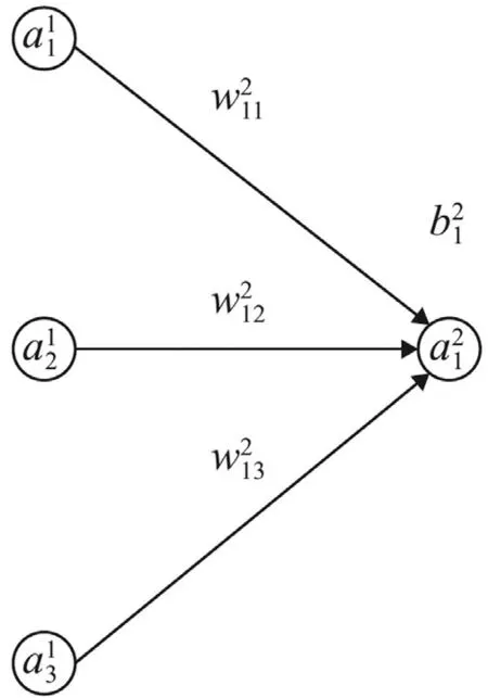
Fig.1. Building block for FFNN.

The structure in Fig.1 refers to a function

The activation function is commonly chosen as the Sigmoid function

or the rectified linear unit (ReLU) function

Please refer to Figs.2 and 3,respectively.Their derivatives areσ(z)(1 −σ(z))for the Sigmoid function,and the Heaviside function for the ReLU function.

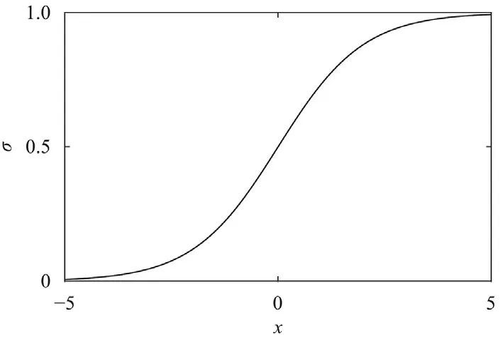
Fig.2. Sigmoid function.

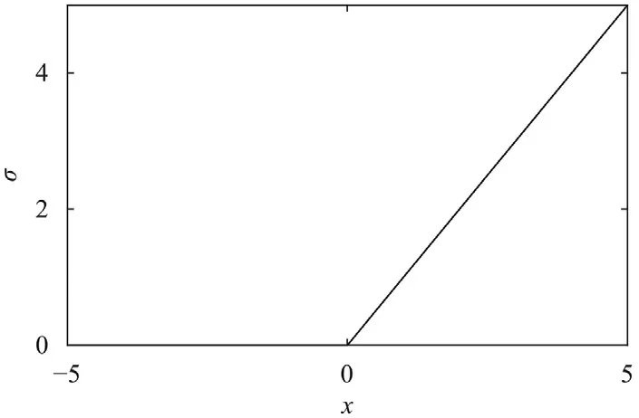
Fig.3. ReLU function.

A general neural network comprises a number of aforementioned building blocks,as illustrated in Fig.4.A neuronis identified by its layer (ℓ∈{1,2,...,L}),and numbering (j∈{1,2,...,nℓ})in theℓ-th layer.For the sake of clarity,we do not mark the weightsand biasesin the figure.Notice that the number of neurons varies from layer to layer in general.In this example,the first layer contains only one neuron.So does the last layer with.These two layers are called as the input layer and output layer,respectively.All layers in between are referred to as hidden layers.

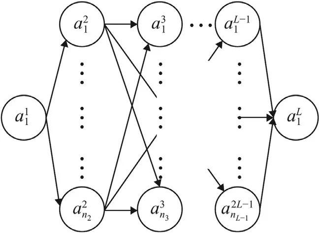
Fig.4. An example of FFNN.

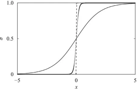
Fig. 5. Sigmoid function with different scalings:solid for σ(z),dotted for σ(10z)and dashed for σ(100z).

Same as before,a neuron at a later layer attains its value from neurons in the precedent layer,i.e.,

with

We notice that usually the same activation function is used over the whole neural network,except that the output layer in general is free of activation function (in another word,uses the identity function).

Universal approximation theorem

Now we demonstrate that for any given continuous function and accuracy tolerance,we may construct an FFNN with specific weights and biases to approximate it.To be specific,in this part we take the Sigmoid function as activation function.

To this end,we plotσ(z),σ(10z),σ(100z)in Fig.5.It is observed thatσ(wz)approximatesH(z)to any desired accuracy,so long aswis chosen big enough.We illustrate withw100 in the following discussions.

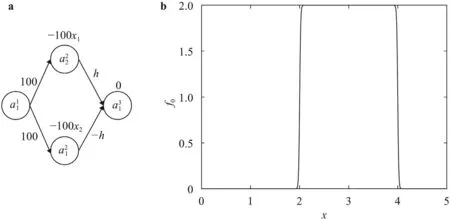
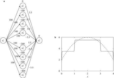
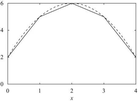
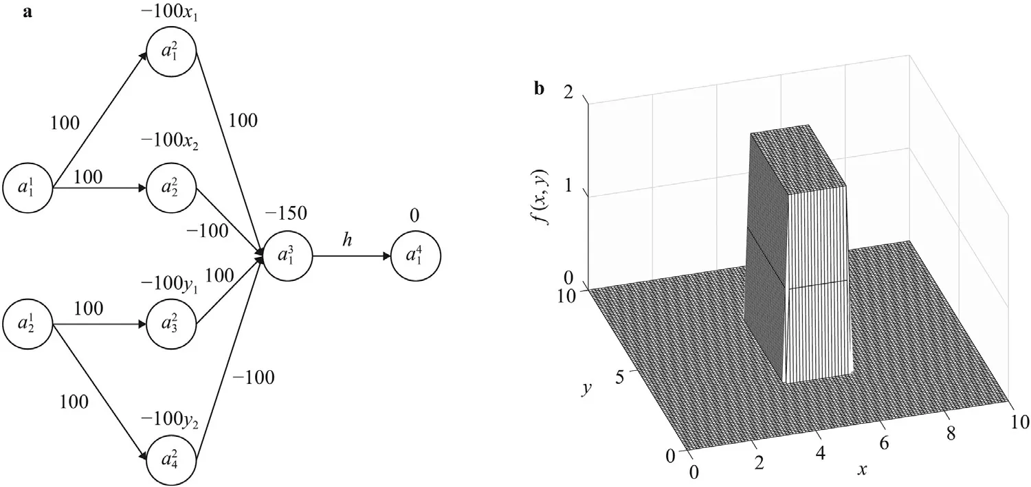
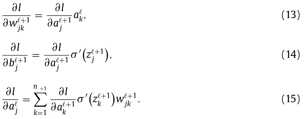
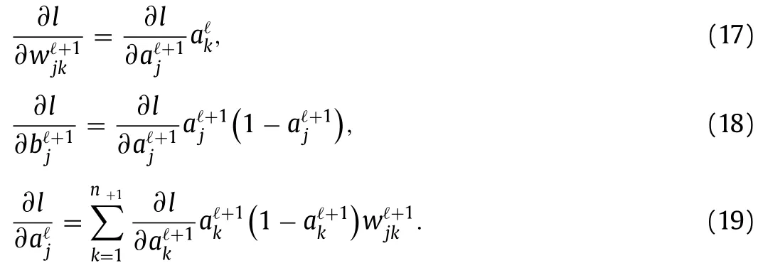
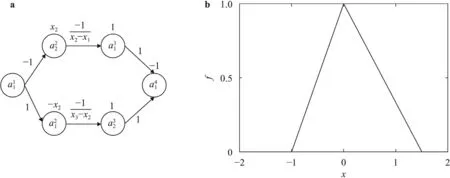
Next,take any two pointsx1

This is realized by a neural network segment in the subplot(a) of Fig.6,withf0(x).The resulting functionf0(x)is shown for a specific casex12,x24,h2 in subplot (b).

Now,piling such segments together,we construct a neural network to represent a piecewise constant functionf(x)which equals tohiwithin(xi,xi+1)for alli.As an illustration,we display a neural network in subplot (a) of Fig.7,to give a piecewise constant functionf(x)in subplot (b).With the input neuronx,the output neuron givesf(x),aiming at approximation of a target functionϕ(x)2+4x−x2over the interval [0,4].

Of course,the currentf(x)is a poor approximation.However,from Calculus we know that every continuous function may be approximated by a piecewise constant function to any desired accuracy,so long as the partition is fine enough.Therefore,with enough many neurons in the hidden layer,we can manipulate the weights and biases to reach the accuracy tolerance.In a more general setting and with a more rigorous arguments,this is termed as the universal approximation theorem [3,4].

Fig.6. Segment of FFNN to represent a square pulse function: a FFNN segment; b f0(x).

Fig.7. Use FFNN to represent a piecewise constant function φ(x),with a goal to approximate a given function ϕ(x)2+4x −x2 in [0,4]: a FFNN; b resulting function f(x)(solid) and the target function ϕ(x) (dashed).

We further illustrate the capability of FFNN in approximating a multi-variate function.Inspired by the single variable function case,we only need to construct an FFNN segment representing a piecewise constant function.To be specific,we consider

In fact,it may be approximated by a compound function

wherewis chosen big enough,e.g.,100.By FFNN in Fig.8,we realize this compound function withw100.The input neurons arex,y,and the output givesf(x,y).The subplot(b) corresponds to a specific choice ofx14,x26,y13,y27,h2.

Fig. 10. Use FFNN based on finite element shape function to approximate a given function ϕ(x)2+4x −x2 in [0,4]:resulting function f(x) (solid) and the target function ϕ(x) (dashed).

It is worth mentioning that a neural network with multiple hidden layers is usually called as a deep neural network.So this FFNN is a deep one.

Backpropagation algorithm

The above constructed FFNN examples illustrate the capability of neural networks in approximating functions.As a matter of fact,it is training procedure instead of explicit construction,that makes neural networks so powerful.

Starting with an FFNN with suitably big number of layers and suitably big number of neurons in the hidden layers,we iteratively update the weightsand biasesFor the single variable case,we take a training setT{(xs,ys)|s1,2,...,S} to minimize a loss function

Fig.8. FFNN segment to represent a piecewise constant function in two space dimensions: a FFNN segment; b resulting function f(x,y).

with a typical choice

Heref(x;stands for the FFNN output under hyperparametersMore precisely,for a given functionyϕ(x),we selectSpointsx1,x2,...,xS,and evaluate their valuesy1ϕ(x1),y2ϕ(x2),...,ySϕ(xS).In a training process,we optimize the hyper-parameters so as to make the difference between true data and FFNN predicted data as small as possible.

The crucial and most expensive step in the optimization,regardless of whatever method is adopted,is the evaluation of the gradient,namely,derivatives ofLwith respect to the hyperparameters.Notice that it suffices to compute the derivatives ofl,and the outputfor each pointxs.We have

On the other hand,from Eqs.(5) and (6),we compute with chain rule that

As mentioned before,the Sigmoid function has a simple form for evaluating derivativeσ′(z)σ(z)(1 −σ(z)).So we obtain

Accordingly,for the data point(xs,ys),we first do a forward sweep,namely,plug inxs,and calculate valuesrecursively fromℓ1 throughL.Then we do a backward sweep,starting from Eq.(12),forℓL−1 through 1,compute

This is referred as a backpropagation algorithm,sometimes abbreviated as BP algorithm.

BP algorithm is advantageous over direct/forward gradient evaluations in terms of operation count.In addition,Eq.(10) implies a data-wise computation for the overall gradient;and for each data point,BP algorithm may be naturally implemented in a vector/matrix fashion albeit nonlinear operations (multiplication) involved.Accordingly,it well suits parallel computing with GPU’s.

Neural network based on finite element shape function

Recently,we proposed a new type of neural network that incorporates finite element shape functions [5].The key idea is to construct an FFNN building block that approximates linear shape function.

Take the ReLU function Eq.(3) as the activation function.Linear shape function on the interval [x1,x2] may be recast in a compound function form.

It is realized by FFNN in Fig.9.

Fig.9. FFNN building block to realize a linear finite element shape function.

As this produces piecewise linear functions,we may stack a number of such building blocks to approximate continuous function as well.See Fig.10 for an illustration to approximate the functionϕ(x)2+4x−x2.A nice feature of this approach is the adaptivity of nodal point position,becausexi’s may be taken as hyperparameters as well.

Conclusions

Neural networks form a new paradigm for scientific computing.The universal approximation theorem elucidates their capability in representing functions.In this tutorial,we constructed FFNN’s to represent piecewise constant functions,both single variable and multivariate.Backpropagation algorithm considerably expedites the evaluations of gradients,hence makes training process feasible to find optimal hyper-parameters.The algorithm is naturally scalable,particularly fits GPU computations.We also present a finite element shape-function-based neural network structure,which readily applies to computational mechanics.

By FFNN,the capability of neural networks in approximating functions has been demonstrated.Other types of networks have also been developed over the years,usually with more hidden layers,including CNN (convolutional neural network),RNN (recurrent neural network),ResNet (residual network),etc.More hidden layers lead to a deeper network,and allow larger capacity for representations.There is yet limited rigorous results about how depth and width influence the performance of a neural network,and how to define the optimal architecture for scientific computing or general applications.Toward substantial understanding and wide applications,much work has been done,and much more is needed.

DeclarationofCompetingInterest

The authors declare that they have no known competing financial interests or personal relationships that could have appeared to influence the work reported in this paper.

Acknowledgments

This work was supported in part by the National Natural Science Foundation of China (Grants 11521202,11832001,11890681 and 11988102).We would like to thank Prof.Guowei He for stimulating discussions.