Experimental Investigation and Simplified Prediction Model Study of Internal Solitary Wave Forces on FPSO

,,,

(1.State Key Laboratory of Ocean Engineering,Shanghai Jiao Tong University,Shanghai200240,China;2.Collaborative Innovation Center for Advanced Ship and Deep-Sea Exploration,Shanghai 200240,China;3.Jiangsu University of Science and Technology,Zhenjiang 212000,China)

Abstract:The forces exerted by internal solitary waves(ISWs)on FPSOwere investigated.A series of depression ISWs were generated by a double-plate wave maker in a density stratified two-layer fluid within a 30-meter-long wave flume.The forces on a fixed FPSO model were measured.Combined with the laboratory experiments,a numerical flume taking the applicability of ISWs theories into consideration was adopted to study the force components.Based on the experimental data and the force composition,the theoretical simplified prediction model for FPSO ISW loads was established.It is shown that the horizontal load consists of two parts:the Froude-Krylov force,which can be calculated by integrating the dynamic pressure induced by ISW along the FPSO wetted surface,and the viscous force,which can be obtained by multiplying the friction coefficient C f,correction factor K and the integration of particle tangential velocity along the FPSO wetted surface.The vertical load is mainly the vertical Froude-Krylov force.It is concluded from the experimental results that the friction coefficient C f and correction factor K are regressed as a relationship of Reynolds number Re,Keulegan-Carpenter number KC and layer depth h1/h.Moreover,the friction coefficient C f follows the natural logarithmic function with Re,while the correction factor K follows four power function with KC number.The force prediction was also performed based on the regression formulas and pressure integral.The predicted results agree well with the experimental and numerical results.The maximum forces increase linearly as the ISWs amplitude increases.Besides,the upper layer thickness has an obvious influence on the extreme value of the horizontal forces.

Key words:internal solitary wave(ISW);FPSO;wave forces;laboratory experiment;friction coefficient and correction factor

0 Introduction

Internal solitary waves(ISWs)exist widely on the continental shelves or slopes[1-3],and have been detected frequently in coastal oceans and marginal seas[4-9]with the development of ocean observing instrumentation.The ISWs can be very energetic with remarkable amplitudes,the largest one of which is 170 m as observed in the South China Sea[10-11].Due to the balance between nonlinear and dispersive effects[4,12],they can keep their shape and speed during the propagation of hundreds of meters below the pycnocline or thermocline.While encountering an ocean engineering structure that serves as a drilling/storage/production platform or wind turbine foundation,the ISWs will exert considerable forces on that equipment and cause serious damage,such as cable breakage,hull rotation,ship collision,etc.[4,13].How to estimate the ISWs-induced forces is an important issue in the design and manufacture of ocean equipment.

Great efforts have been devoted to obtain accurate wave forces over the recent decades.The fundamental laws are acquired from the study on cylinder structures,by adopting the Morison’s empirical formula[14-19].Platforms with more complicated geometries[20],like Spar,semi-submersible and tension leg(TLP),are considered the combinations of cylinders.Their ISW forces on different parts,like columns,horizontal and diagonal braces,can be estimated by adopting the Morison’s empirical formula with modified coefficients.Huang et al[21]and Chen et al[22]presented good examples in their works in which two sets of modified coefficients were developed through model experiments and data fitting for the Morison empirical formula.Wang et al[23]also developed a numerical flume to obtain satisfying calculation resultson the ISWs forces.

However,it is noticed that the ISWforce problem of FPSOhas not been fully discussed yet,although the force is also a very important type of the oil platform.Previous work from Xu et al[24]and Zhang et al[25-26]shows that the FPSOhas a very different structure from those of the platforms mentioned above,so its ISW force cannot be calculated by using Morison’s empirical formula based on cylinder components.How to estimate the ISWforceson a FPSOplatformisa new problem.

To solve such a problem,a series of laboratory experiments were conducted in a stratified flume to measure the forces exerted by ISWs on an FPSO.Meanwhile the numerical simulation was carried out in a numerical flume to clarify the composition of ISWs forces on an FPSO.Chapter 1 in this paper gives the brief description of the experimental configuration and numerical flume,followed by discussion of the analysis of experiments and numerical simulations.In Chapter 2,a simplified prediction model of the ISWs forces on FPSO is deduced from the experimental data.Finally,conclusionsare drawn in Chapter 3.

1 Experimental investigation

1.1 Experimental equipment

The laboratory experiments were carried out in a wave flume of 30 m long,0.6 m wide and 1.2 m high in Shanghai Jiao Tong University.Two-layer fluid of fresh and brine water was prepared by using the two-bucket method.The flume was filled with fresh water to a desired depth,then the brine water was injected slowly beneath the lighter fresh water through two openings on the bottom of the flume until the total water depthhreached 1.0 m.The density of the fresh and brine water wasρ1=998 kg/m3andρ2=1 025 kg/m3,respectively.The thickness of the upper layer(fresh water)wash1and that of the lower layer(brine water)wash2.A typical density profile is shown in Fig.1(a).The buoyancy frequencyNwas calculated byN=[(g/ρ1)(∂ρ/∂z)]1/2,whereρ=ρ(z)is the density andgis the gravitational acceleration.The vertical distribution is shown in Fig.1(b),in which a narrow pycnocline can be seen.The interface between the upper and lower layer is the plane of the maximumbuoyancy frequency.

Fig.1 Two-layer fluid system of h1/h2=1/4

The sketch of the experimental facility is plotted in Fig.2.For the reference coordinate system,its origin is located at the start point of wave on the interface.Thexcoordinate directs to the wave propagation direction while thezcoordinate directs upward.The wave maker wasequipped to generate ISWs in the two-layer system,which followed the mechanism described by Huang et al[27].The ISW profile was recorded using two arrays of conductivity probes,which were placed at pre-arranged positions along the flume.The first array was set atx1=10.2 m and the second one was set atx2=13.2 m.Each array included 13 vertically-arranged conductivity probes with a 3 cm spacing.Fig.3 shows the ISWprofile in experiments,and Fig.4 shows the ISWprofile recorded by conductivity probes array.The phase speed of ISW followsc=Δx/Δt,in whichΔx=x2-x1is the distance between two arrays andΔtis the time lag of wave peaks.A wave absorption facility is fixed downstream to avoid the wave reflection.

Fig.2 Sketch of the experimental set-up

Fig.3 ISWprofile in experiments

Fig.4 ISWprofile recorded by conductivity probe array

The 1:400 FPSOmodel was used in the experiments.The main parameters are presented in Tab.1.The model was stiffly mounted atx=13.9 m below a rigid frame and the draft isd=0.035 m.A threecomponent force transducer was fixed between the FPSO and the rigid frame to measure the forces exerted by a depression ISW.The electrical signals representing the force variation on the FPSOwere recorded.The relationship between the force and signal were calibrated before the experiment.

The sketch of the numerical experiments is plotted in Fig.5,which is consistent with the laboratory flume.The computational domain consists of 3 zones to generate,propagate and absorb the ISW.The entire domain is divided into 2 018 440 hexahedral structured cells while the wetted surface of the FPSO is divided into 3 688 facets.The VOF(volume of fluid)method is employed to track the interface of the two-layer fluid.The sponge layer method is adopted to absorb the ISW at the end of the numerical flume.

Tab.1 Principal dimensionsof the FPSO(Unit:m)

Fig.5 Sketch of the numerical flume

wherecisthe phase velocity,andζis the interface displacement calculated by ISWtheory.

Due to the feasibility of the ISW theory,the nonlinear parameter is defined asε=|a|/h，the dispersion parameter is defined asμ=(h/λ)2,whereλis the characteristics length,h=h1+h2is the total depth of calculation flow field,andais the ISWamplitude.For a given ISW,the nonlinear parameterεand dispersion parameterμfor the KdV,eKdV and MCC ISW equations are calculated respectively.The KdV equation[28-29]is selected forμ＜μ0andε≤μ,whereμ0=1 is the critical dispersion parameter summarized by experiment data.The eKdV equation[5,30-31]is suitable forμ＜μ0andμ≤ε≤μ1/2.Besides the situations above,MCCequation[32]is the right choice.

1.2 Experimental forces

The characteristic length of the FPSO modelLwlis chosen as the immersed windward area per unit depth.HereLwl=0.51 m.As shown in Tab.2,Lwlis much smaller than the ISWwavelengthL,i.e.Lwl/L≤0.2 forh1/h2=20/80 and 15/85,so that the influence of the model on the incident wave field is negligible,not forh1/h2=10/90.It should be noted thatLis the measured wavelength of the generated ISW instead of the characteristic lengthλ.The ISW wavelengthLis actually infinite in the theory,so we choose the length where the ISWheight reaches 5%of the amplitude in the experiment.

Tab.2 Summary of the ISW wavelength L and L wl/L

The measured ISW amplitudes are adopted for numerical simulations.The results of experimental and numerical dimensionless horizontal/vertical forces exerted by ISW on FPSO model are shown in Fig.6 with three different upper-lower layer thickness ratios.The numerical results agree well with the experimental results.Only a few discrepancies are observed at the trough of the curve.Those may result from the variation of the pycnolcline,since each experiment attempt will slightly change the stratification and decrease the accuracy of the theoretical phase speed calculation.

Fig.6 Experimental and numerical dimensionless horizontal/vertical forces

Fig.7 Time history of dimensionless horizontal/vertical ISWforces when h1/h2=15/85,||a/h=0.088

Fig.8 Time histories of dimensionless horizontal/vertical load components with h1/h2=15/85,||a/h=0.088

By taking the case withh1/h2=15/85,|a|/h=0.088 as example,the velocity profile with horizontal and vertical distribution is shown in Fig.9.The particle horizontal velocity direction is consistent with the propagation direction of ISW in the upper layer fluid,but opposite in the lower layer fluid.Thus a horizontal shear flow is generated on the wave surface.Moreover,a vertical flow can be induced by the ISW at the wave surface.The particle vertical velocity is downward in the front of the ISW trough,but upward behind the ISW trough.Therefore,flow rotation happens at the ISW trough.

As the ISW propagates to the FPSO,there appears a high pressure zone at the stem of FPSO,as shown in Fig.10.Moreover,two lower pressure zones are found at the FPSOstern and the bottom bow of FPSO.Furthermore,vortices are observed in the lower pressure zones.These vortices cause the viscous pressure force of FPSO.But through the previous analysis,the viscous pressure force is a small amount and can be negligible.

Fig.9 Distribution of flow velocity induced by ISW

Fig.10 Distribution of pressure and velocity around FPSOwhen t=62 s

2 Simplified prediction model establishment

On the basis of the investigation above,wave pressure difference force is caused by the particle fluctuation and can be calculated by Froude-Krylov formula

According to Bernoulli equation,the instantaneous dynamic pressurepinduced by ISW is expressed as[21]

whereuiandwiare the horizontal and vertical instantaneous velocity of water particles induced by ISW.

In this study,experimental data are used to investigate the friction and viscous pressure difference coefficients.The horizontal wave pressure difference force can be calculated based on pressure integration following Eq.(2).Deducting the horizontal wave pressure difference force from the measurements,the rest is the sum of the horizontal friction and viscous pressure difference forces,which is called the viscous force.Viscous pressure difference force has a strong dispersion because of unsteady vortex around FPSOand cannot be measured precisely.By introducing a correction factorK,the viscous pressure difference force can be calculated based on the friction force.Thus,the viscous force can be integrated with the tangential velocity induced by ISWalong FPSOwetted surface and is expressed as

According to the feasibility of ISWtheoretical models,Eq.(4)is adopted to calculate the horizontal viscous force of the FPSO.By comparing the calculated results with the experimental and numerical results,the friction coefficientCfand correction factorKare obtained by the least square method.

The friction coefficients and correction factor majorly depend on the Reynolds numberRe,Keulegan-Carpenter numberKC,hull form and roughness of the FPSOsurface.HereReandKCare defined asRe=UmaxLwl/υandKC=UmaxT/Lwl,in whichUmaxrepresents the maximum horizontal velocity induced by ISWs,andTis the ISW period.In addition,it is found thatCfandKare also related to the upper layer thicknessh1/h.

The relationship between the friction coefficients and the Reynolds numberReis determined through comparative analysis,as shown in the left sub-picture of Fig.11.The solid points represent the experimental values of the friction coefficient while the hollow marks represent the numerical values.The friction coefficientCfdecreases with the increasing Reynolds number in the reciprocal of the natural logarithmic function forRe=25 000～70 000.The fitting curve is determined through regression analysis and the simplified prediction formula ofCfcan be written as

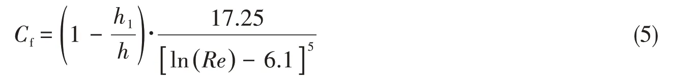
Since the viscous pressure difference force is related to the eddies of particle,the correction factorKis mainly related to theKCnumber.The right sub-picture of Fig.11 shows the relationship between correction factorKand theKCnumber under different cases.The correction factorKfirst decreases and then increases with increasingKCnumber forKCfrom 0.45 to 1.2.By fitting the scatter points from the experiment or the computation,the simplified prediction formula ofKis expressed as

Fig.11 Friction/viscous pressure difference coefficients versus Re and KC,here A=45.5(2.2KC-1.75)4 in the right subpicture

The performance of the simplified prediction model on the total horizontal force is shown in Fig.12.The prediction result agrees well with the experimental and numerical data.Only slight differences occur at the peak and valley of the curves.Generally,the simplified model is satisfying in prediction of the horizontal force.It should be noted that some oscillations occur in the experimental profile after the valley because of the trailing wave trains.The characteristics of such small waves are still not clear now,so their prediction may depend on the further efforts on thisproblem.

Fig.13 shows the vertical force profile from different methods.In the simplified prediction model,the vertical force is calculated by pressure integral on the wetted surface of FPSO along the depth direction.The predicted vertical force is well consistent with the experimental and numerical results.Three force profiles are generally the same besides the trailing waves in the experiment.Therefore,the prediction model is proved effective,which combines the regression formulas and pressure integral with coefficient and correction factor that are determined experimentally.

Fig.12 Time history of the dimensionless total horizontal forces

Fig.13 Time history of dimensionless vertical force

Fig.14 demonstrates the extreme values of the horizontal forces from different methods under different ISW amplitudes and layer depth ratios.For the horizontal forces,the maximums increase with the increasing ISW amplitude while the minimums generally tend to decrease but with some exceptions.If the depth ratio becomes smaller,the maximums obviously grow larger while the minimums roughly grow smaller.The reason is that a smaller depth ratio makes the pycnocline and ISW closer to the FPSO,so that the forcesmust be larger.

Fig.14 Horizontal force extreme values of experimental,numerical and simplified prediction formula results

For depth ratioh1/h2=10/90,the trend of minimum values with the ISWamplitude is different from the other two cases.The reasons of this difference are still not clear now,so it is worth making further efforts on smaller depth ratio cases.

The extreme values of the dimensionless vertical forces under different ISW amplitudes and depth ratios are shown in Fig.15.The predicted vertical forces agree well with the experimental and numerical results.The vertical forces nearly increase linearly with the increase in ISWamplitude.Additionally,the dimensionlessmaximum vertical forces are hardly affected by the layer thicknessratio.

One more point that may be noticed in Fig.14 and Fig.15 is that the differences between the measured and the predicted results become more significant when the amplitude grows larger.The reason is that in the experiments,large amplitude ISWs are always performed later than the small ones.After several attempts,the mixing of the two layers makes the pycnocline thicker,diverging from the restrict two-layer assumption in the prediction model.

Fig.15 Comparison of vertical force extrema between experiments,numerical simulation and simplified prediction formulas

3 Conclusions

In order to establish the simplified prediction model for ISW forces,experiments are conducted to measure the total forces exerted by ISWs on FPSO,and numerical simulation are adopted to clarify the forces components.The generated and simulated ISWs are recorded and applied to the simplified prediction forces’calculation.The main conclusions are drawn asfollows:

(1)The general observations have been made by comparing experimental forces with the numerical forces.The simulated results agree well with the measurements.The clarified components for ISWs forces are believable,which is that the horizontal forces are dominated by the wave pressure difference force.However,the horizontal viscous force cannot be ignored because of the viscosity effect of fluid.For the vertical ISWs forces,only the wave pressure difference force is calculated.

(2)Regression formulas of the friction coefficientCfand newly introduced correction factorKin simplified prediction formulas are established based on the experimental data.The friction coefficient decreaseswithRenumber in thenatural logarithmic functionCf=( 1-h1/h){17.25/[ln(Re)-6.1]5},while the correction factor varies withKCnumber in four power function 10h1/h·K=(1-h1/h)6·[5.65+33.3·(2.2KC-1.75)2-45.5·(2.2KC-1.75)4].The predicted forces by regression formulas and pressure integral are well consistent with the measured and simulated results.

(3)The ISWforces increase nearly linearly with the ISWs amplitude.The maximum horizontal forces increase with the upper layer thickness decreasing,while the ISWamplitude and upper layer depth have great effects on the minimum horizontal forces.The influence of layer thickness on the vertical forcesis negligible.

In this paper,the density of stratified fluid and the ISWpropagation direction are selected as a result of referring to the related laboratory experiments of internal solitary waves[28,33-34].The experimental results,including the variable law of ISWforces and the effects of the amplitude or the layer depth on the forces,have a certain reference value for marine structure design.In the real ocean,the loads induced in a continuous stratified fluid by ISWs with more variable propagation direction,which is more similar to the real ocean,will be the next step of our research.