Remaining Useful Life Prediction for a Roller in a Hot Strip Mill Based on Deep Recurrent Neural Networks
2021-06-18RuihuaJiaoKaixiangPengandJieDong
Ruihua Jiao, Kaixiang Peng,, and Jie Dong
I. INTRODUCTION
HOT rolling is one of the most widely used processes in steel production. The roller is the most important tool in hot rolling production, since its quality and service life directly affects the stability of strip production and can further influence the production efficiency. Once the roller is damaged, it will not only lead to the fracture of the strip, but can cause a fire due to the high temperatures of more than 1000 °C during the rolling process. The roller is a consumable part, so it should be maintained every day. However, as quality requirements of products continue to increase, higher demands are placed on the use of rollers. As a consequence,maintenance strategy should shift from traditional breakdown maintenance and preventive time-based maintenance to condition-based maintenance (CBM), which is also called predictive maintenance (PdM) or prognostics and health management (PHM) [1].
PHM is an engineering process of failure prevention, and remaining useful life (RUL) prediction [2]. The core process of PHM is to make reliable predictions of the RUL [3], [4].The RUL of a roller refers to the lifetime left on the component from the current time to end-of-life (EoL).Accurate RUL prediction is able to provide helpful information for the management of rollers. It can not only guarantee the surface quality of the hot rolled products and avoid losses caused by accidental failure of the roller, but it also improves the operating rate of the rolling mill so as to increase production efficiency of the business. Therefore,accurate RUL prediction for rollers is of great significance for the production of hot rolling, and special attention needs to be paid to the design of a reliable and accurate RUL prediction approach.
Generally, the existing RUL prediction methods can be classified into three categories: model-based, data-driven, and hybrid approaches [5]. The basic idea of the model-based method is to develop a mathematical model that can describe the physical characteristics and failure modes of the system to realize the prediction of the RUL. It usually achieves more accurate results but cannot be applied to systems that lack prior knowledge about the physical degradation. The widely used model-based approaches include the Paris-Erdogan model [6], the Kalman filter [7], and the particle filter [8].Data-driven methods are able to construct a mapping relationship between input and output based on a large amount of historical data and then predict the RUL, which can avoid the disadvantages of model-based method. A large number of data-driven approaches, such as the autoregressive model [9],the proportional hazard model [10], the Wiener process [11],the support vector machine (SVM) [12], and the artificial neural networks [13], have been studied in the past few years and have made remarkable achievements. By combining several of the aforementioned methods, hybrid approaches are able to leverage advantages of different models while avoiding their disadvantages at the same time [14]. For instance, Weiet al.[15] proposed a framework that integrates SVM and particle filter to estimate the RUL of batteries,which not only provides a possible failure time range, but also improved the accuracy of prediction results compared with conventional methods. In [16], the particle filter algorithm is introduced to estimate the state of Wiener process to remove the influence of multisource variability and survival measurements. However, developing an effective and reliable hybrid approach still remains challenging, in particular the combination of model-based and data-driven methods.Accordingly, a new hybrid approach is proposed in this paper.
Recently, since the multilayer deep network architecture can fully capture the representative features from original measured data, deep learning methods have been widely used in many fields, such as speech recognition, image recognition,and fault diagnosis [17]. It has also been gradually applied to the field of PHM. In [18], an enhanced restricted Boltzmann machine was proposed to construct a heath indicator (HI), and the RUL of the machines were estimated through a similaritybased method. The experimental results demonstrate the advantages of the proposed method. Liet al.[19] proposed a data-driven method based on a deep convolution neural network for RUL prediction, where accurate prediction results can be obtained without prior knowledge and signal processing. Compared to the previously mentioned deep network architecture, the recurrent neural network (RNN) is a more effective approach for processing time-series data since they have an internal state that can represent aging information [20]. Heimes [21] presented a RUL prediction model based on the RNN for turbofan engines, which won the 2008 PHM competition. Guoet al.[22 ] proposed a HI construction method based on RNN for predicting the RUL of bearings, where the experiment showed that the approach has better performance than some other methods. These applications indicate that the RNN-based approach has enormous potential for PHM and RUL prediction.
In the hot strip production process, the roller is in direct contact with the metal to be rolled in order to plastically deform the metal. Due to the large rolling force of the hot strip mill (HSM), the friction between the work roller and the rolled metal is extremely high. Accordingly, wear becomes the major factor affecting the service life of the rollers [23].With the increase of rolling time, the wear degree gradually increases, which will cause the surface of the roller to become rough, requiring maintenance of the component. The traditional theory of roller RUL prediction is based on the prediction of wear. However, there are still some lacunae which are worth discussing. First, these theories are based on an empirical model and only consider central influencing factors such as rolling pressure, contact arc length, and rolling length, which is a simplification of the real situation. At present, there still does not exist an accurate prediction model based on the wear mechanism. Oike’s equation [24] is a widely used empirical model. However, it cannot predict the wear precisely when applied to different industrial sites. In[25], a roller force model was integrated with Oike’s equation to estimate the wear along the roller barrel, and the accuracy of prediction was improved. Secondly, the traditional model requires some important parameters, such as the coefficient of friction and the uneven friction coefficient of the steel plate,which are unmeasurable quantities in industrial cases.Although the empirical relationships between these coefficients and other measurable parameters, like rolled material, strip temperature, and lubrication, can be derived,these relationships are sometimes contradictory [26]. Thirdly,it is unreasonable that the RUL of the roller be determined only by the degree of wear. Roller deformation, roller fatigue,mechanical factors, and the processes of rolling also affect the service life of the roller. It is difficult to establish a mathematical model to describe the relationship between these factors and the RUL.
In order to overcome these shortcomings in predicting the RUL of rollers, a new method which can extract coarsegrained and fine-grained characteristics to estimate the health state and predict the RUL is proposed in this study. To form a feature set that contains various roller degradation characteristics for accurate RUL prediction, the coarse-grained and fine-grained characteristics are extracted from batch data based on the proposed deep RNN. Then, the features are used to construct a HI that is capable of indicating the health state of the roller. Following that, the RUL can be estimated by extrapolating the HI model, which is described by a double exponential function, to a predefined failure threshold (FT).Finally, the effectiveness of the proposed method is verified by the dataset collected from an industrial site.
For the approach proposed in this work, the main contributions and innovations are:
1) The proposed deep RNN architecture is able to extract coarse-grained features from monitoring data and fine-grained features from maintenance data to develop a comprehensive HI that can reflect the health state of the roller. Furthermore,the model parameters can be obtained automatically during network training, rather than the model parameters of traditional methods are sometimes unmeasurable.
2) The RUL of the roller is determined by the developed comprehensive HI rather than relying on just one factor as in the conventional method, which is more reasonable. In addition, the constructed HI has a value equal to one under fault state, so there is no need to artificially specify a FT.
3) A RUL prediction and health state estimation framework based on deep RNN is proposed for the RUL estimation of the roller of HSM, where many monitored variables related to the roller wear that are not considered by empirical models are taken into account in this work.
II. PROPOSED DEEP RNN NETWORK ARCHITECTURE
A. Basic Theory of Recurrent Neural Network
As a kind of deep learning approach, RNN is well suited for dealing with sequential data. This can be attributed to the special network structure that remembers previous information and applies it to the calculation of the current output. As shown in Fig. 1, at timet, the input of the hidden layer comes not only from the input layerxt, but also from its own output at the previous momentht−1. As a result, the outputytis determined by both the present input information and the information at timet−1.

Fig. 1. Structural diagram of the RNN.
The RNN is generally trained using a back-propagation through time (BPTT) algorithm. However, as the time information stored in the RNN increases, the gradients tend to vanish or explode [27]. In order to overcome this problem, a long short-term memory (LSTM) network architecture including memory cells is proposed [28]. The memory cell is introduced to replace the hidden neuron in the hidden layer of a traditional RNN. It records the information for a long time through a forget gate, an input gate, and an output gate. There is an initial cell state in the memory cell, which is assigned with certain unit weight. All components of the LSTM are shown in Fig. 2.
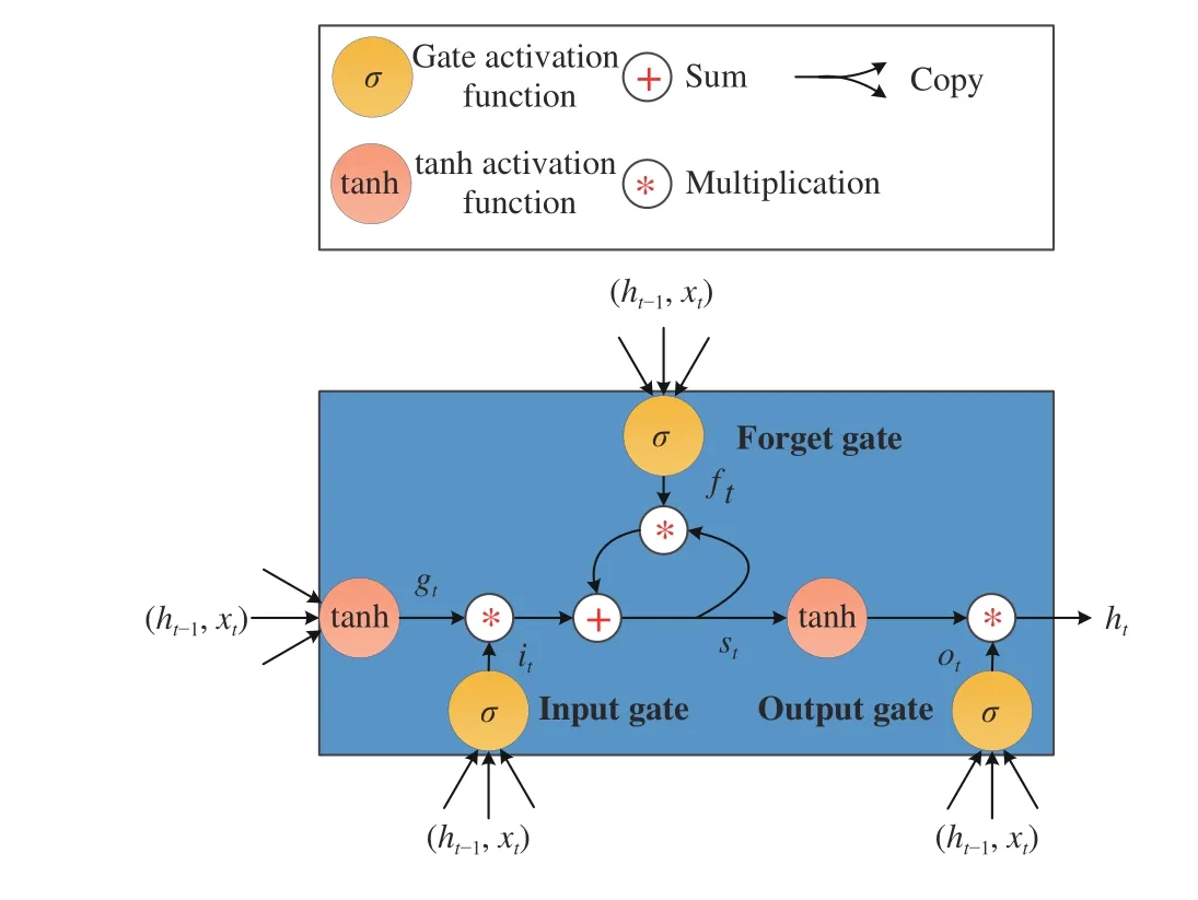
Fig. 2. The network architecture of the LSTM memory cell.
Forget Gate:The forget gateftis used to decide how much information will be discarded. With a sigmoid layer, it outputs a number between 0 and 1, where 1 indicates the cell state value is fully reserved and 0 represents the value is completely forgotten. The forget gate can be calculated as

Input Gate:The input gateitis used to determine what new information is to be stored in the cell state and to update the cell state. This step consists of two parts. First, a sigmoid layer is used to update the input value. After that, a tanh layergtis used to create a candidate state, which can be multiplied by the input value to update the cell state. These can be implemented as

With (1)–(3), the current cell state can be updated as

Output Gate:The output gateotis introduced to decide which information will be output. First, a sigmoid layer is used to determine which part of the cell state will be output.Then, the remaining state value can be obtained by multiplying the outputs of a tanh layer and the sigmoid layer.This can be calculated as

B. Proposed Network Architecture
The hot rolling process is a typical batch process, which produces strip steel coil-by-coil and each coil represents a batch [29]. Considering that the HSM production process has its own unique characteristics, it is necessary to design a targeted modeling method. The HSM can be used to produce a wide range of products in different materials, shapes, and sizes, and different products inevitably lead to different wear rates. The HSM processes a large number of products by continuously repeating the rolling operation. Thus, a certain periodicity may exist between each batch of the monitored data. In view of the above characteristics, a deep RNN model is proposed that can fully extract the fine-grained features from the monitoring data and the coarse-grained features from the maintenance data. The monitoring data refers to the data collected during the rolling process, which contains approximately 180 measuring points in each batch. Thus, finegrained features can be used to model wear rate under different working conditions. The maintenance data refers to the data collected after rolling a batch of steel, where each batch of steel contains only one measurement point. Thus,coarse-grained features can be used to model the periodicity of rolling. The network architecture consists of three substructures, i.e., a multilayer LSTM for extracting finedgrained features which is represented as LSTM1, a multilayer LSTM for extracting coarse-grained features which is represented as LSTM2, and a fully connected layer for regression. Fig. 3 shows the network architecture of the proposed approach.

Fig. 3. The architecture of the proposed deep RNN.
First, the collected data is prepared as input data for the LSTM in 3-dimensional (3D) format for the convenience of training. The dimension of the data isNs×Ntw×Nid, whereNsis the number of samples,Ntwindicates the time window, andNiddenotes the number of selected input dimension.
Afterwards, the multilayer LSTM1 is developed to extract fine-grained features from the monitoring data, and the multilayer LSTM2 is constructed to extract coarse-grained features from the maintenance data, which can both learn the most suitable feature representations from each raw input data. After model convergence, each vector of the outputs in the two multilayer LSTMs naturally represents the finegrained and the coarse-grained features, respectively.
Finally, all the extracted features are connected to a fully connected layer, and one neuron as a representative of the output is added at the top of the network for HI estimation. To further improve the performance of the proposed deep RNN,the Adam algorithm [30] is used to optimize the neural network. In addition, the dropout [31] technique is used to regularize the hidden layers, which is able to alleviate overfitting and improve generalization ability. The parameters of the deep RNN model are optimized to minimize the error between the actual HI and the estimated HI.
III. REMAINING USEFUL LIFE PREDICTION
A. Health Indicator Construction
In order to develop a comprehensive HI to assess the health state of the roller, the proposed deep RNN is used to fuse the fined-grained features and coarse-grained features as the HI.Specifically, in the training step, a label set indicating the percentage of roller degradation at timetis attached to the input data set. Thus, the HI can be expressed as

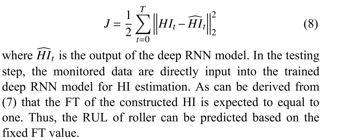
whereHItrepresents the label at momentt, andTis the number of steel batches rolled during the last maintenance to the next maintenance. For example, assuming that the roller maintenance time is after rolling 380 batches of steel, and the current monitoring time point is the 228th batch of steel, then the label HI is 0.6. Accordingly, the deep RNN model is trained to minimize the cost function as follow:
B. Remaining Useful Life
For the purpose of estimating the RUL, the double exponential model is introduced to describe the HI model,which has been proved to be an effective model for RUL prediction [27]. Thus, the state-space model can be built as follow:

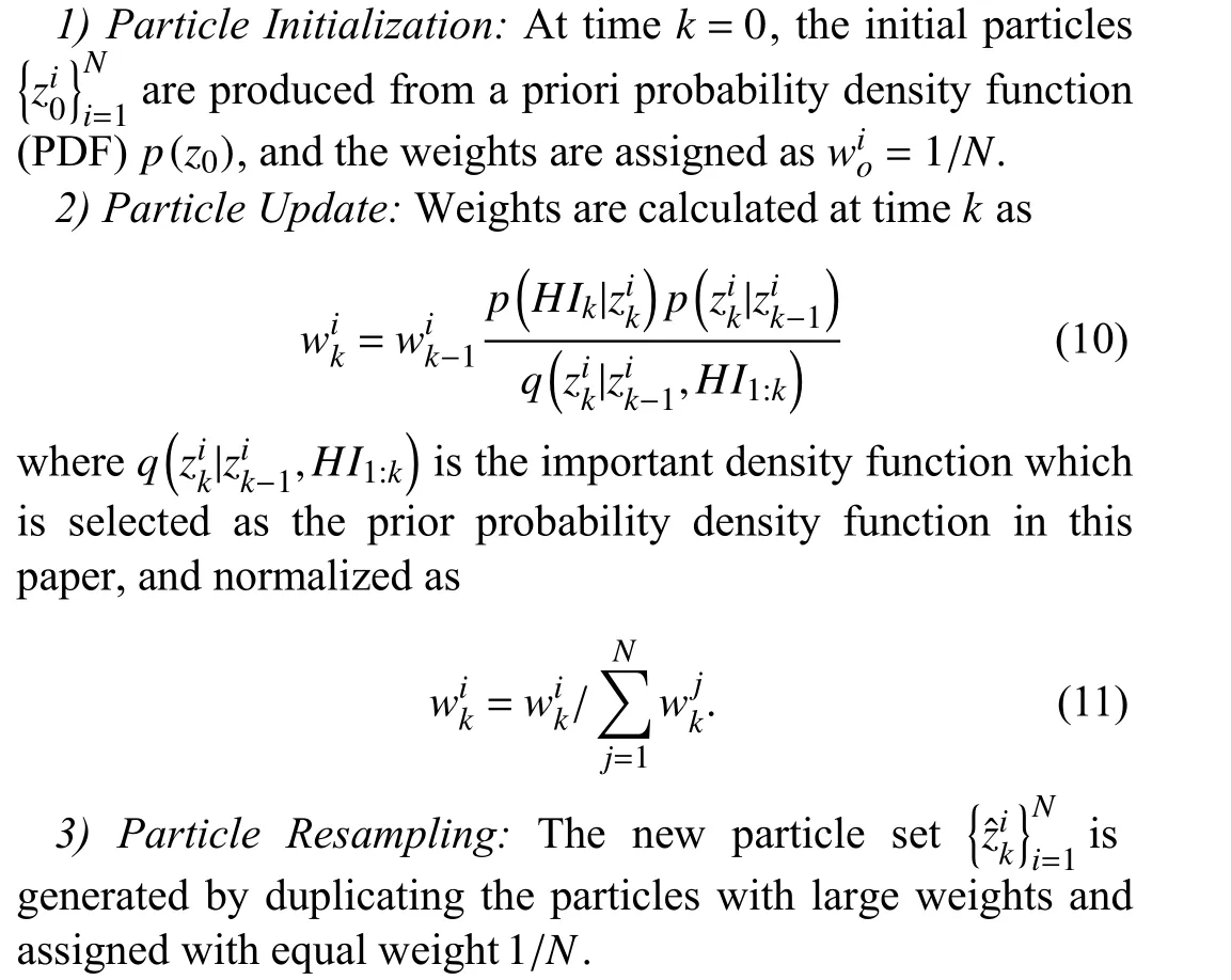
The particle filter (PF) algorithm is used to predict the future HI based on this state-space model. The main idea of PF is to sample a large number of random particles using the Monte Carlo method, and give each particle an importance weight to represent the posterior probability density. More details about PF can be found in [32]. The PF algorithm includes the following four steps:
4) State Estimation:The new state is calculated by using new particles and weights as

Once thetmeasurements of the HI have been obtained, the posterior PDF of the state variable at timetcan be derived with the particle states as
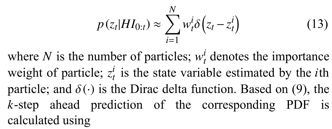

and the prediction value of the state is

Accordingly, the HI can be predicted by substituting (15)into (9). Suppose thatLitis the failure time that is estimated by theith particle, which can be calculated by extrapolating the state-space model until the HI exceeds the predefined FT for the first time. Thus, the RUL associated with theith particle is obtained as follows:

and the PDF of the RUL prediction is further can be estimated by

The whole process of the proposed RUL prediction framework is shown in Fig. 4.
IV. EXPERIMENTAL STUDY: APPLICATION TO THE HSM
A. Descriptions of the HSM
The modern hot strip rolling process is a very complex process, and it is able to customize production based on order.In general, the hot strip rolling process consists of six subprocesses as shown in Fig. 5 [33]. The steel slab is first heated in the reheating furnace to about 1200 °C–1280 °C, then it is rolled back and forth in the roughing mill until the thickness of the slab reduces to the desired thickness for the finishing mill. After being passed through the transfer table, the thickness and width are shaped as expected in the finishing mill. Following that, the extremely hot strip steels are cooled by a laminar cooling system, and then the cooled strip is coiled for the convenience of storage. The finishing process is the core of the hot strip rolling line, and the control function of product quality is mainly concentrated in this area.Therefore, the work roller of the finishing mill will serve as the focus in this work.
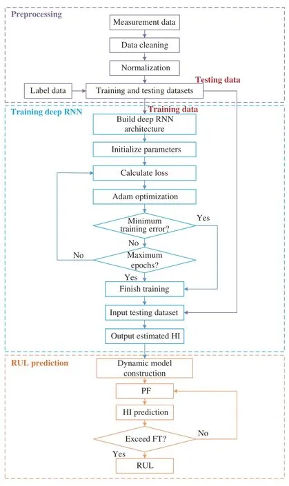
Fig. 4. Flowchart of proposed RUL prediction framework.
The experimental data set was collected from the HSM of a 1700-mm hot rolling line in March 2019. It is generally believed that the rollers have reached the end of their service life and need to be replaced after rolling a large number of batches of steel. The work roller maintenance data of the last stand were collected during 12 cases of maintenance, and the corresponding rolling monitored data were also collected.Among them, 10 of the collected data sets were treated as the training set, and the other two were used to test the performance of the proposed method.
B. Data Preprocessing
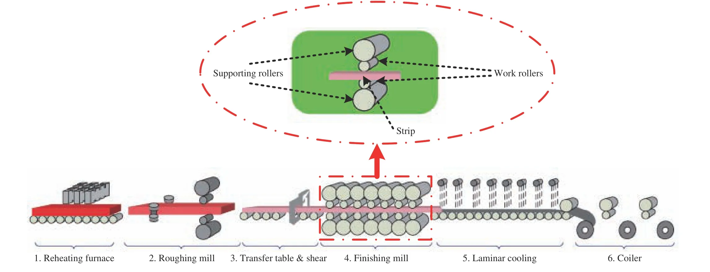
Fig. 5. Schematic of the hot strip rolling process.
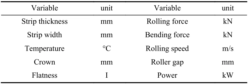
TABLE I DETAILED DESCRIPTIONS OF VARIABLES FOR LSTM1

TABLE II DETAILED DESCRIPTIONS OF VARIABLES FOR LSTM2
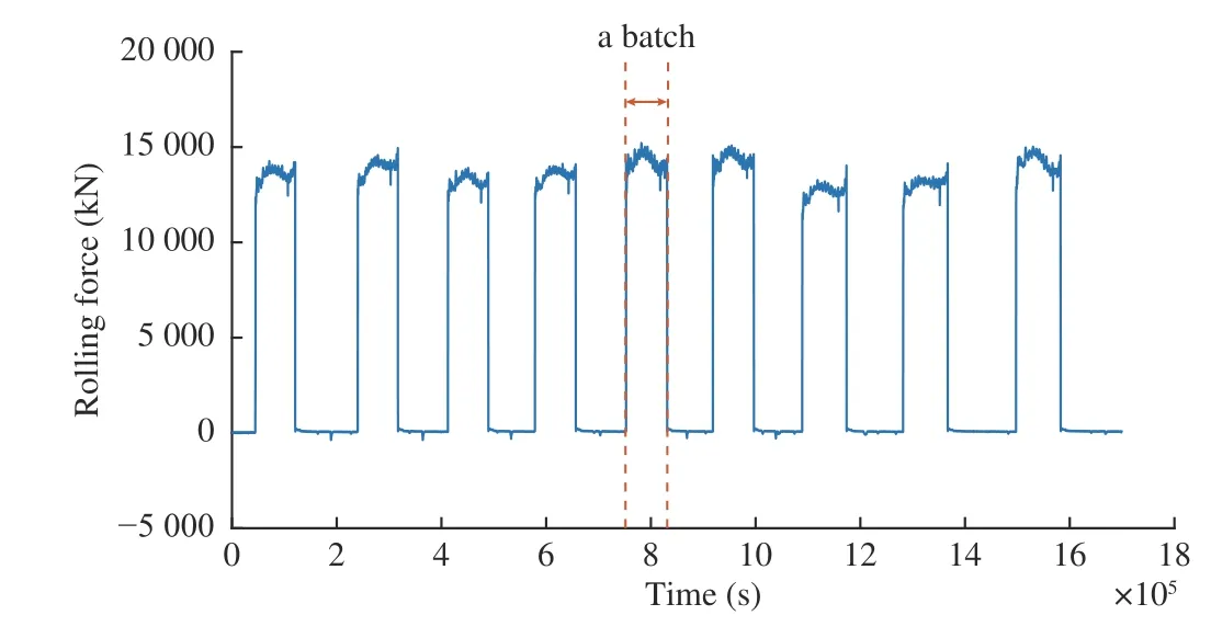
Fig. 6. An example of a monitoring sample of the rolling force.
Fifteen variables were used in total. Ten of them were input to LSTM1 as shown in Table I, which are collected during the rolling process. The other five variables collected after rolling a batch of steel were used as the input for LSTM2, and the detailed descriptions are shown in Table II . Due to the difference in rolling time for each batch, as shown in Fig. 6,the monitoring data for LSTM1 should be trimmed to the same length. Since the data lengths have little difference, the shortest batch data could be found out from all modeling data,and then the data of remaining batches were cut to this length.In addition, the value of each variable was normalized using min-max normalization to eliminate the dimensional effect between the variables.
C. Experimental Setup
In the proposed deep RNN, the network structure parameters strongly depend on the complexity of the problem.Considering the complexity of the research problem and the number of available training samples, the LSTM1 for finegrained feature extraction was set to have five LSTM layers which contain 128, 200, 256, 360, and 512 hidden nodes,respectively, and the LSTM2 for coarse-grained feature extraction was set to three LSTM layers with 32, 64, and 128 hidden nodes, respectively. The truncated BPTT with the minibatch stochastic gradient descent method was used to update the weights during training, and Adam optimization algorithm was used to optimize the neural network. In the testing phase, once the collected test data set is input into the deep RNN, the network outputs a HI corresponding to the health of the roller as the recognized result. A detailed configuration of this deep RNN is summarized in Table III,and all the parameters were selected based on a large number of trials.

TABLE III DETAILS OF DEEP RNN
D. Results and Discussion
1) HI Construction Results:In order to quantitatively evaluate the constructed HI, two metrics of monotonicity(Mon) and correlation (Corr) [34] are considered here. The monotonicity metric is used to evaluate the tendency of an HI,and a higher score means a better performance in monotonicity, which can be calculated by

whereTrepresents the length of the HI during the lifetime;d/dHI=HIT+1−HITis the difference of the HI sequence;Num o f d/dHI>0 andNum of d/dHI<0 are the number of the positive differences and the negative differences,respectively.
The correlation metric is able to reflect the correlation property between HI and operating time, which is denoted as


According to (18) and (19), the Mon and Corr of the proposed approach are obtained and listed in Table IV. To demonstrate the advantages of the proposed HI construction method, an RNN was modeled for comparison using the multilayer LSTM1 for fine-grained feature extraction, which is denoted as RNN1. Another RNN with multilayer LSTM2 for coarse-grained feature extraction was also used to construct a HI for comparison, and marked as RNN2.

TABLE IV HI CONSTRUCTION RESULTS
It can be seen from Table IV that the Mon and Corr values of deep RNN and RNN1 are both larger than RNN2, and the deep RNN achieves the highest values. The large values imply that the HI established by deep RNN has a better performance in monotonicity and correlation. Through the comparison, it is demonstrated that the proposed deep RNN network structure which can extract fine-grained and coarse-grained features has better performance than other RNN-based methods.
2) RUL Prediction Results:To verify the effectiveness of the proposed RUL prediction approach based on deep RNN,the two collected test sets, represented as test01 and test02,were used for prediction and analysis. Due to the statistical properties of the PF algorithm, the estimation results are in distribution forms approximated by 5000 samples. The RUL of test01 was estimated on the 161th and 242nd batch, and the estimation and prediction results are shown in Fig. 7. The mean of the HI prediction is indicated by the blue line, and the 95% confidence interval (CI) for HI estimation and prediction are also given. Fig. 7(a) shows the EoL predicted at the 161th batch, which means that the data from the first 161 batches are used to update the model. Thus, the RUL and 95% CI can be derived based on (16) and (17). From Fig. 7(c), it can be seen that the median value and 95% CI of RUL are 37 batches and[31, 47], respectively, which indicates that roller maintenance is required after rolling 37 further batches of steel. As shown in Fig. 7(b), the HI estimated for test01 at the 242nd batch exceeded the FT at the 252nd batch. The RUL prediction results are shown in Fig. 7(d), and the 5th, 50th, and the 95th percentiles of the RUL are 5, 10, and 17, respectively.
The estimation and prediction results for test02 are shown in Fig. 8, which are estimated on the 195 th and 263 th batch. As shown in Fig. 8(a), the estimated HI at the 195 th batch is higher than FT for the first time at batch 223, indicating that the EOL is 223 batches. The PDF of the RUL is shown in Fig. 8(c), the median value and 95% CI of RUL are 28 batches and [22, 35], respectively. As can be seen from Fig. 8(b) that the EoL predicted at 263 th batch is 277 batches, and the PDF of the RUL is plotted in Fig. 8(d). The 5 th, 50 th, and the 95th percentiles of the RUL are 7, 14, and 21, respectively, which indicates that it is necessary to maintain the rollers after rolling 14 more batches of steel.
The comprehensive results of the prediction performance are listed in Table V. It can be seen that the RUL prediction results with long available batch data for both test01 and test02 are more accurate than those with shorter ones. This can be attributed to the limitation of the Bayesian method. If there is no new measurement information to update the model,the prediction accuracy will decrease as the prediction window increases. On the other hand, the uncertainty of the rolling schedule and the uncertainty in the actual rolling process can also lead to the inaccuracy of the initial predictions. However, once new measurement data are acquired, the parameters of state-space model are automatically updated to improve the prediction results. Although the prediction at the beginning is imprecise, the prediction results become more and more accurate as the measured data increases.
In order to further demonstrate the advantages of the proposed deep network architecture, convolutional neural network (CNN) and deep belief network (DBN) are used for comparison. The CNN has five convolution layers, and a fully connected layer is also added at the end so as to have the same architecture as deep RNN. The DBN is composed of four restricted Boltzmann machines, and the basic neural network is attached at the top layer. The approaches are carried out on the two test datasets, and root mean square error (RMSE) and mean absolute error (MAE) are used to assess the performance, which are defined as
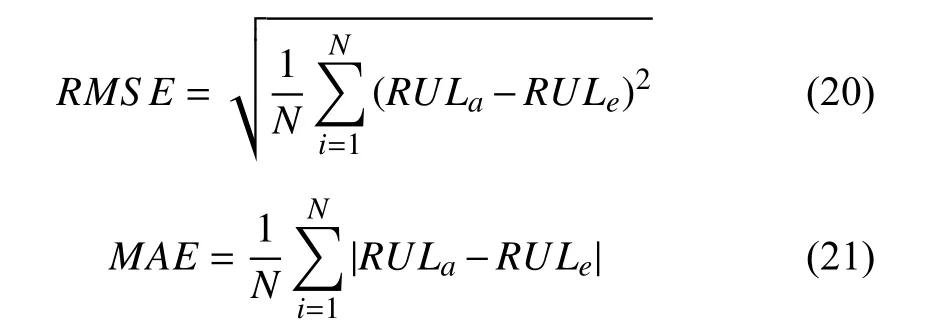
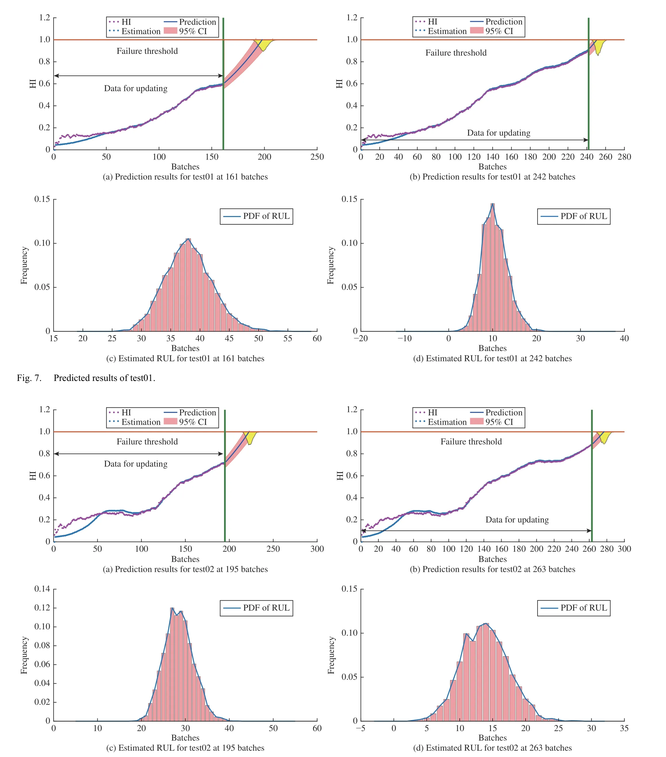
Fig. 8. Predicted results of test02.
whereRULais the actual RUL value; andRULeis the estimated value.
The comparison results with respect to the RMSE and MAE are summarized in Table VI . RNN2 achieves the highest RMSE value, which indicates its prediction error is the largest. The RMSE values of RNN1, CNN, and DBN are 17.67, 18.97, and 15.23, respectively, which are higher than the deep RNN. Deep RNN achieves relatively low MAE valueas 9.85, while the MAE values of RNN1, RNN2, CNN, and DBN are 15.42, 26.25, 15.74, and 14.37, respectively. From the results, it is observed that the deep RNN has the smallest prediction error. This demonstrates that the deep RNN network structure proposed in this study is able to extract coarse-grained and fine-grained features to construct the HI,and can further accurately predict the RUL for rollers of HSM. Furthermore, the prediction result based on the proposed RUL framework include a time range of possible failures, which can provide more useful information for roller management decision.

TABLE V RUL PREDICTION RESULTS

TABLE VI COMPARISON OF THE PREDICTION RESULTS
V. CONCLUSION
Rollers plays a significant role in the hot rolling process.With their wide and frequent application in steel production,the RUL prediction of rollers has become a crucial and challenging issue. To solve this problem, a deep learning architecture based on RNN was developed to estimate the RUL in this work. Firstly, a deep RNN model was established to extract the coarse-grained and the fine-grained features to construct the HI. Afterwards, the PF algorithm was introduced to iteratively update the parameters of a constructed statespace model, and the PDF of RUL could be estimated by extrapolating the dynamic model to the FT. In the end, the proposed methods were applied to the HSM to predict the RUL of the rollers. The proposed RUL prediction framework is helpful for the management of the roller, since it can effectively reduce the production cost and improve the operating rate of the HSM so as to improve the production efficiency of the business.
The following conclusions can be drawn from the experimental results. First, the proposed deep RNN network structure is able to extract coarse-grained and fine-grained features to create the HI. Second, the developed comprehensive HI is able to reflect the health of the roller, and it gradually increases with the deterioration of health state.Third, compared with some other popular deep learning methods, the proposed RUL prediction framework is able to accurately predict the RUL for rollers of HSM since it obtained relatively low RMSE and MAE values.
Despite the good experimental results achieved by the proposed approach, it still needs further optimization in the future. On one hand, the parameters in the deep network structure can be further optimized through some optimization algorithms, such as [35] and [36]. On the other hand, some efforts should be made to improve the PF so as to obtain higher prediction accuracy.
杂志排行
IEEE/CAA Journal of Automatica Sinica的其它文章
- Disassembly Sequence Planning: A Survey
- A Cognitive Memory-Augmented Network for Visual Anomaly Detection
- Human-Swarm-Teaming Transparency and Trust Architecture
- Lightweight Image Super-Resolution via Weighted Multi-Scale Residual Network
- Towards Collaborative Robotics in Top View Surveillance: A Framework for Multiple Object Tracking by Detection Using Deep Learning
- Global-Attention-Based Neural Networks for Vision Language Intelligence
