Speed and Accuracy Tradeoff for LiDAR Data Based Road Boundary Detection
2021-06-18GuojunWangJianWuRuiHeandBinTian
Guojun Wang, Jian Wu, Rui He, and Bin Tian
Abstract—Road boundary detection is essential for autonomous vehicle localization and decision-making, especially under GPS signal loss and lane discontinuities. For road boundary detection in structural environments, obstacle occlusions and large road curvature are two significant challenges. However, an effective and fast solution for these problems has remained elusive. To solve these problems, a speed and accuracy tradeoff method for LiDAR-based road boundary detection in structured environments is proposed. The proposed method consists of three main stages: 1) a multi-feature based method is applied to extract feature points; 2) a road-segmentation-line-based method is proposed for classifying left and right feature points; 3) an iterative Gaussian Process Regression (GPR) is employed for filtering out false points and extracting boundary points. To demonstrate the effectiveness of the proposed method, KITTI datasets is used for comprehensive experiments, and the performance of our approach is tested under different road conditions. Comprehensive experiments show the roadsegmentation-line-based method can classify left, and right feature points on structured curved roads, and the proposed iterative Gaussian Process Regression can extract road boundary points on varied road shapes and traffic conditions. Meanwhile, the proposed road boundary detection method can achieve real-time performance with an average of 70.5 ms per frame.
I. INTRODUCTION
IN the autonomous vehicle (AV) field, environmental perception is a prerequisite for other functional modules,and road boundary detection is an important part of this perception. Road boundary can be used to distinguish on-road area from non-road area, which provides an important basis for AVs to understand scenes and make decisions. In addition,when GPS data is inaccurate, or perhaps has been lost in an urban environment, the road boundary can be used as an effective feature to locate AV. Therefore, accurate and reliable road research communities have invested much time into this area. According to sensors, current methods can be divided into vision-based and LiDAR-based methods.
With the development of computer vision technology,vision-based methods are widely used in road boundary detection [1]-[3]. Effective detection results can be achieved using vision-based methods, but performance is greatly affected by light and weather conditions. In addition, it is difficult to obtain accurate depth information, which makes it difficult to meet the needs of autonomous driving applications.
Compared with vision sensors, LiDAR can provide the accurate depth information and is immune to illumination and shadow. Thus, LiDAR has become an indispensable sensor for AV at this stage. In [4], the method based on the 2D-LiDAR interactive multi-model was used to detect road boundaries. In[5], road boundary points were extracted as line segments in polar coordinates based on 2D-LiDAR. However, due to the sparsity of 2D-LiDAR data, it is difficult to meet the needs of environmental perception. Compared with 2D-LiDAR, 3DLiDAR has the advantages of a 360-degree scanning range,which can provide a large quantity of data, known as point cloud, and thus plays an increasingly important role in AV. In previous the Defense Advanced Research Projects Agency(DARPA) challenges, many teams used 3D-LiDARs for environmental perception [6], [7]. In recent years, Waymo,Baidu, and other companies have chosen 3D-LiDAR as the main sensor to obtain environmental information [8]-[10].
Although 3D-LiDAR has many advantages, there are still two great challenges for road boundary detection: the classification of road boundary points on curved roads and obstacle occlusions. On curved roads, it is difficult to distinguish left and right boundary points even if all boundary points are extracted, which also has an important effect on autonomous driving safety. Besides, when obstacle occlusions exist, false points caused by obstacles will also affect road boundary detection.
In order to solve these problems, we propose a speed and accuracy tradeoff method to extract road boundaries from the point cloud. The proposed method can filter out false points caused by obstacles under non-congested traffic conditions and can correctly classify left and right boundary points on curved roads. The main contributions of this paper are as follows:
1) This paper presents a road-segmentation-line-based classification method for classifying feature points. The feature points are rough road boundary candidate points extracted by spatial and geometrical features. The road segmentation line is determined by a beam band model and an improved peak-finding algorithm. The method can classify left and right feature points accurately on curved roads up to 70 m away.
2) This paper proposes a distance filter and random sample consensus (RANSAC) filter for candidate point extraction and seed point extraction. The candidate points and seed points would be used for the subsequent feature points filtering based on an iterative Gaussian Process.
3) This paper proposes an iterative Gaussian Process Regression (GPR) based feature points filtering method. The GPR algorithm can be applied to various road shapes without assuming that road boundaries are parametric models. At this same time, the algorithm can effectively remove false points caused by obstacle occlusions. Because GPR is a nonparametric model, it significantly enhances the adaptability to various road shapes and the robustness for obstacle occlusions.
The road-segmentation-line-based classification method and the iterative GPR effectively addressed the problem of curved road and obstacle occlusions in structured environments. The proposed road boundary detection method achieves excellent accuracy while ensuring real-time performance.
The remainder of this paper is organized as follows. Section Ⅱdescribes a review of related research. Section Ⅲ introduces the methodologies for road boundary detection. Section Ⅳpresents comprehensive experiments and evaluations. Section V summarizes the major contributions of this research, and its future work is presented.
II. RELATED WORK
A. Related Work on Feature Points Classification
For the classification of left and right road boundary points,most of the existing literature focuses on the problem of straight road structures in which left and right boundary points are classified just according to lateral coordinates, such as in[11]-[15]. Xuet al. [16] extracted feature points based on energy functions and classified left and right boundary points using the least-cost path model. This method can work well on curved roads, but it requires manual addition of source points,making this algorithm unusable in practice. In [17], super voxels were used to obtain boundaries, and then trajectory data was used to classify left and right boundary points, which can only work offline and are not suitable for on-line applications. In [18] and [19], in order to solve the problem of boundary detection on curved roads, clustering methods were proposed to divide left and right boundary points. However,these methods need to iterate at each possible segmentation angle to maximize the classification score, which requires a lot of computation. In [20], road boundary points are searched and separated by the predicted trajectory of autonomous vehicles. In this method, the cumulative error of the predicted trajectory would increase, which would affect the accuracy of road boundary points detection. In [21], the parametric active contour and snake model were used to extract the left and right road boundary, and navigation information was necessary to initialize the snake model.
B. Related Work on Feature Points Filtering
For the problem of obstacle occlusions, various filtering methods have been proposed. Sunet al. [11] and Yanget al.[14] firstly classified feature points into segments with knearest neighbor (KNN) method, then segments of less than three points were considered as false points and eliminated,which may filter out true isolated boundary points. In [12], a RANSAC line fitting algorithm was used to filter out false points, which assumed that roads were straight, thus making it not suitable for curved roads. In [15], a regression filter was introduced to make the detection robust to occlusions. In [19],a RANSAC quadratic polynomial fitting algorithm was used to remove false points. References [12], [15] and [19]modeled road boundaries as a linear or quadratic polynomial parameterized model, and were not suitable for various road shapes. In [20], road boundary points are extracted only based on spatial features, which is not enough to remove false points caused by obstacles. In [22], feature points were extracted based on local normal saliency, and distance to trajectory was used to filter out false points that cannot filter out false points inside the road. In [23], region growing-based filtering was used to extract true road boundary points based on the similarity of height and intensity. However, in a structured environment, the materials used for road boundaries and road surfaces are usually the same, and the intensity was not effective. In [24], multiple parameterized RANSAC models were used to extract road boundary points.
III. METHODOLOGY
As shown in Fig. 1, the proposed method consists of four main steps. It takes a frame of raw point cloud as input and outputs road boundary points.
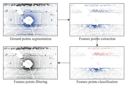
Fig. 1. The pipeline of road boundary detection method.
A. Ground Points Segmentation
The proposed method is used to process point cloud from Velodyne HDL-64E LiDAR [25]. The LiDAR coordinate systems are defined, as shown in Fig. 2. The directions are given from the drivers’ view,X: forward,Y: left,Z: up, and the coordinate system is right-handed. In this paper, we consider the range of [-3, 1] × [-40, 40] × [-70, 70] meters along for theZ-axis,Y-axis,X-axis, respectively as the detection regions for road boundaries.
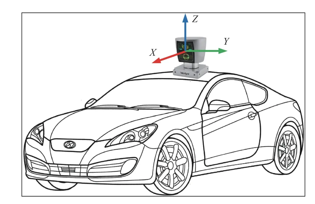
Fig. 2. The cartesian coordinate system of LiDAR.
Since road boundaries are a part of the ground, off-ground and on-ground points can be separated by ground segmentation. In this paper, a piecewise plane-based fitting method is used. For convenience, we usePto represent a frame of raw point cloud. First, point cloudPis divided into several segments along thex-axis. Then, a RANSAC plane fitting method is applied in each segment to extract on-ground points [26]. Because the point cloud is divided into segments,we assume that the slope of the ground in each segment does not fluctuate greatly and can be approximated to a plane.Besides, we focus on road boundary detection, so the ground point segmentation does not require high precision, and the distance threshold is set to 28 cm, which is determined through a trial-and-error method. The distance threshold should ensure that the ground point contains all road boundary points, which generally in the range of 15 cm to 30 cm.
Fig. 3 shows the results of a ground point segmentation,where on-ground points are used to extract road boundary points, and off-ground points are used to compute road segmentation lines for classifying road boundary feature points. For convenience, letPondenote on-ground points andPof foff-ground points. All figures pertaining to point cloud illustrations in this paper are from the top view.
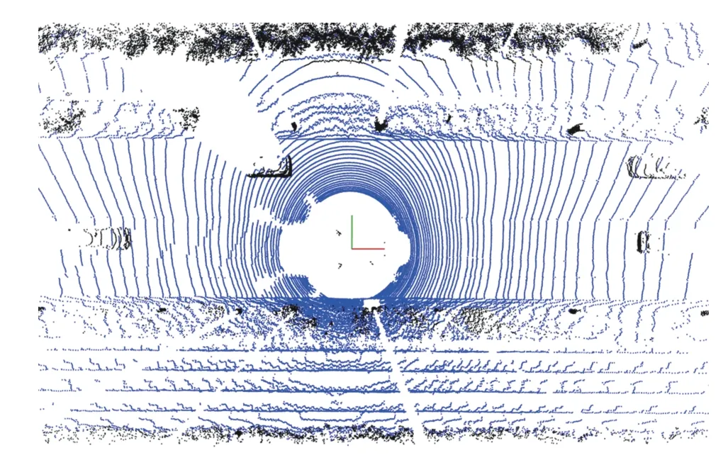
Fig. 3. An example of ground point segmentation. On-ground points are in blue, off-ground points are in black.
B. Feature Points Extraction

3) Horizontal Distance
The horizontal distance feature is proposed by [27] to represent the horizontal distance between two adjacent points in the same layer. It sets a horizontal distance threshold δxy,lto determine whether pointpliis a feature point. It is defined by

whereHsis the absolute value of the height of pointpli, θlis the vertical azimuth of scanning layerl, and θais the horizontal angular resolution of LiDAR. Ifpliis selected as a feature point, the horizontal distance betweenpliand its adjacent points should be smaller than δxy,l.
All the features are tested in experiments, and loose thresholds are determined by a trial-and-error method. The height thresholdsTheight1,Theight2, andTheight3are determined based on the height jump of road boundaries.Theight1andTheight3are generally drawn from [0.01, 0.05], andTheight2is generally drawn from [0.15, 0.35]. The smoothness threshold is determined based on the smoothness of road boundary areas, soTsmoothnessis generally drawn from [0.001, 0.005].
C. Feature Points Classification
In order to solve the problem of classification for road boundary points, especially on curved roads, this paper proposes a road-segmentation-line-based method to classify feature points, which is mainly inspired by [27]. The principle of the method is that the beam model [29] is established based on off-ground pointsPof f, from which the length of each beam is calculated. The longest beams in the front and rear regions of the AV are regarded as road segmentation lines,which indicates the direction of the road. Compared with [27],an improved peak-finding algorithm is proposed to filter out outliers and determine two truly dominant extremes in the distance function δ(k). Thus, the proposed improved peakfinding algorithm in this paper is more robust for the sparsity of point cloud and losses of laser return. Then, feature pointsPfeatureare divided into left and right feature points according to the road segmentation lines. Compared with the clustering methods used in our previous work [19], the proposed method can achieve real-time performance, and it can classify feature points accurately under diverse road conditions.

Fig. 4. Beam model based on off-ground points. The blue lines are middle lines of each beam band.
1) Beam Band Model
The beam model was proposed by Thrun [29] in 2005 and has been widely used in the field of robotics. In order to determine the accurate angle of road segmentation, the angular resolution θmodelof the beam model is set to 1 degree.In classical beam models, the beam length is the distance from the launching point to the nearest point. In this paper, we expand the beam into a beam bandZk

where (xb,yb) is the launching point, which is the LiDAR origin in this paper. The LiDAR scans clockwise, where zero degrees is on thex-axis. (x,y) denotes off-ground points, andk∈{1,2,...,360}. The beam length of each band is defined as the shortest distance of the points in this band to the launching point, that is

(xi,yi)∈(Zk∩Pof f)d(k) δ(k)


where if there is no point in thek-th band, δ(k)=1. So, in order to determine road segmentation lines, especially in roads with large curvatures, the longest beam will be used as road segmentation line in front region ({0 ≤k≤90∪270 ≤k<360}) and rear region ({ 90 ≤k<270}) of the AV. After that,an improved peak-finding method is used to determine the road segmentation line.
2) Improved Peak-Finding Algorithm
The peak-finding algorithm was first proposed to find the number of dominant extremes that represent road direction from aerial images in [30]. For example, Figs. 4 and 5 show a beam model based on off-ground pointsPo f fand corresponding distance function δ(k). It is clear that because point cloud data is sparse, the distance function has many false dominant extremes (δ (k)=1). However, we just need two true dominant extremes to determine the road segmentation line. To solve this problem, we present an improved peak-finding algorithm. The algorithm consists of two steps: the first median filter is applied to process the distance function, then each dominant extreme is evaluated based on the extreme width.
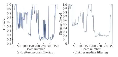
Fig. 5. An example of distance function for beam band model.
a) Median filtering
Median filtering is a nonlinear digital filtering technique which is often used to remove noise from an image or signal[31]. With the beam model established above, a distance function δ(k) is obtained, and each δ(k) is replaced by the median of its corresponding neighbors. Figs. 5(a) and 5(b) are the distance function before and after filtering, respectively.
b) Evaluating dominant extremes based on extreme width
For dominant extreme δ(k), extreme widthwis defined as follows:

whereklis the nearest beam band whose distance δ(kl) is less than δ(k) on the left ofk, andkris the nearest band whose distance δ(kr) is less than δ(k) on the right ofk. The evaluation of dominant extremes is as follows:
i) Remove the dominant extremes whosewis less than a pre-defined thresholdTw
ii) Merge the dominant extremes that are close. For two
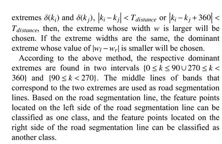
In order to demonstrate the effectiveness of the proposed method, experiments are carried out under three different road curvature conditions, as shown in Fig. 6, the green line represents the road segmentation line, where the left feature pointsPfeature,lare blue, and the right feature pointsPfeature,rare red. We can see that the proposed improved peak-finding method can determine road segmentation lines accurately on different curved roads.

Fig. 6. Results of feature points classification on three different road curvatures. The green line represents the road segmentation line, the left feature points are in blue, and the right feature points are in red. (a) Small. (b)Moderate. (c) Large.
D. Feature Points Filtering
After feature points are extracted and classified, there are still many false points, including vehicles, pedestrians, railway tracks, adjacent roads, and so on. Besides, even on structured road environments, the shape of road boundaries is irregular and cannot be accurately modeled with parametric models.The GPR model is a nonparametric model, which has both powerful approximate and outlier rejection abilities. Based on this, an iterative GPR algorithm is proposed to model road boundary and filter out false points. Before the iterative GPR,a filtering-based method is proposed in this paper to extract candidate points and seed points.
1) Candidate Points and Seed Points Extraction
The filtering-based method includes a distance filter and a RANSAC filter. Feature pointsPfeature,landPfeature,rare filtered by the distance filter to obtain candidate pointsPcandidate,landPcandidate,r, and seed pointsPseed,landPseed,rare obtained by the RANSAC filter.
a) Distance filter:The distance filter is used to remove false points caused by obstacles outside roads. In general, we assume that road boundaries are the nearest obstacle to vehicles. So, the method is to divide feature points into segments based onxcoordinates, and to find the nearest point to thex-axis of LiDAR as a candidate point in each segment:
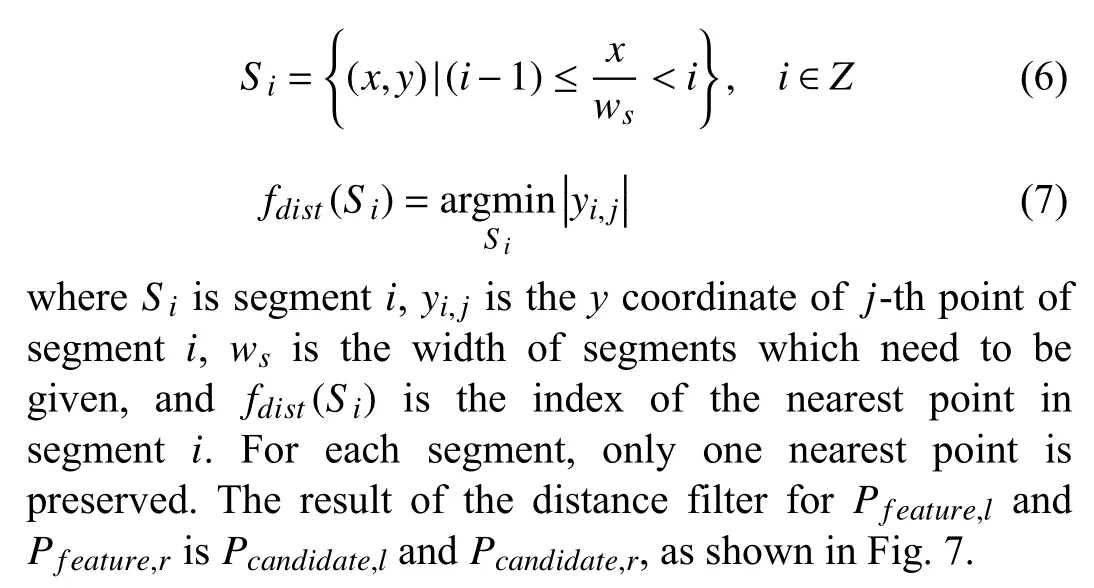

Fig. 7. Candidate points (left is in red, right is in blue).
b) RANSAC filter:In order to extract seed points, the false points caused by obstacles inside roads such as pedestrians and vehicles must be filtered out. The filter models road boundaries as a quadratic polynomial, then a RANSAC algorithm is applied to fit the model [26]. Then, all the points whose distances from the fitted model are less than the threshold are used as seed points. The result of RANSAC filter forPcandidate,landPcandidate,risPseed,landPseed,r, as shown in Fig. 8. It is clear that the RANSAC filter also removes some true boundary points because of the assumption that road boundaries fit a quadratic polynomial model. In order to improve the robustness of road boundary detection, iterative GPR is further applied to extract road boundary points.2) Iterative Gaussian Process Regression
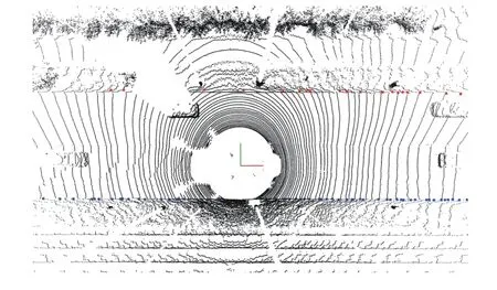
Fig. 8. Seed points (left is in red, right is in blue).
Due to the diversity of road shapes in urban environments, a single parametric model cannot be used to accurately model road boundaries. Besides, there are many false points in candidate points, and iterative GPR happens to have strong outlier rejection abilities. To improve the robustness of the road boundary detection algorithm, this paper proposes to use GPR to model road boundary, which is inspired by [32].
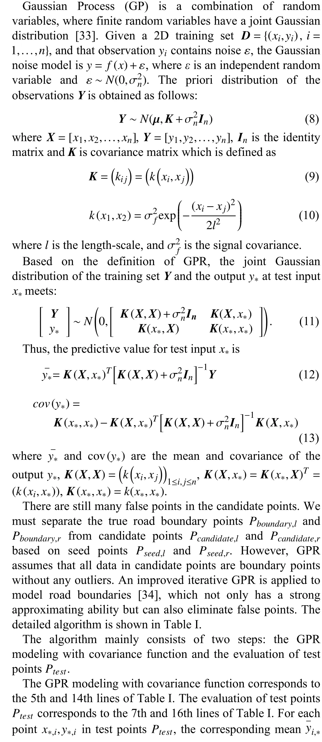
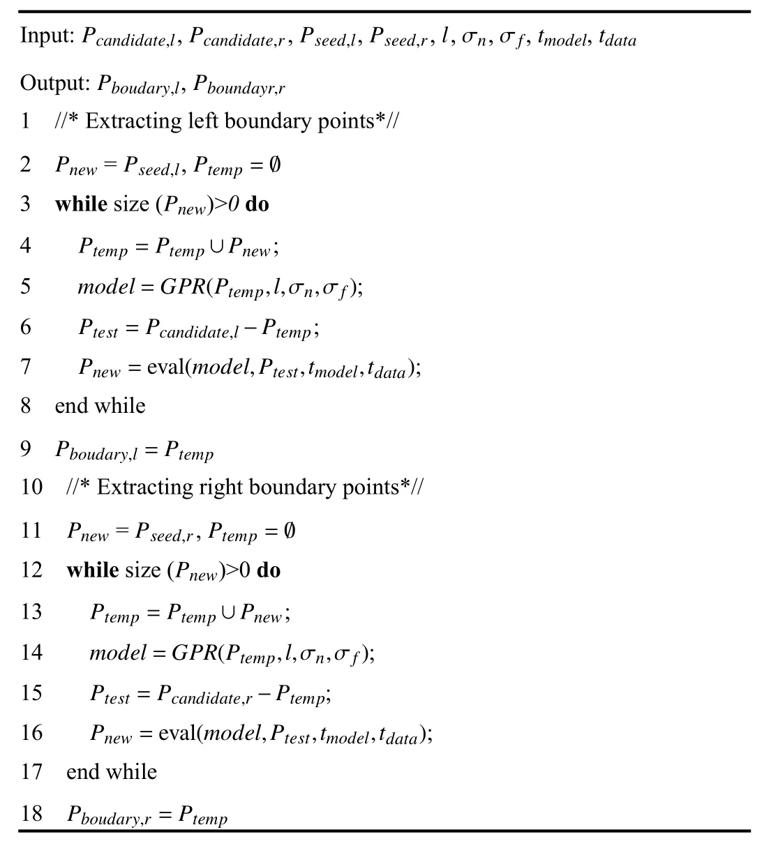
TABLE I BOUNDARY POINTS EXTRACTION BASED ON ITERATIVE GPR
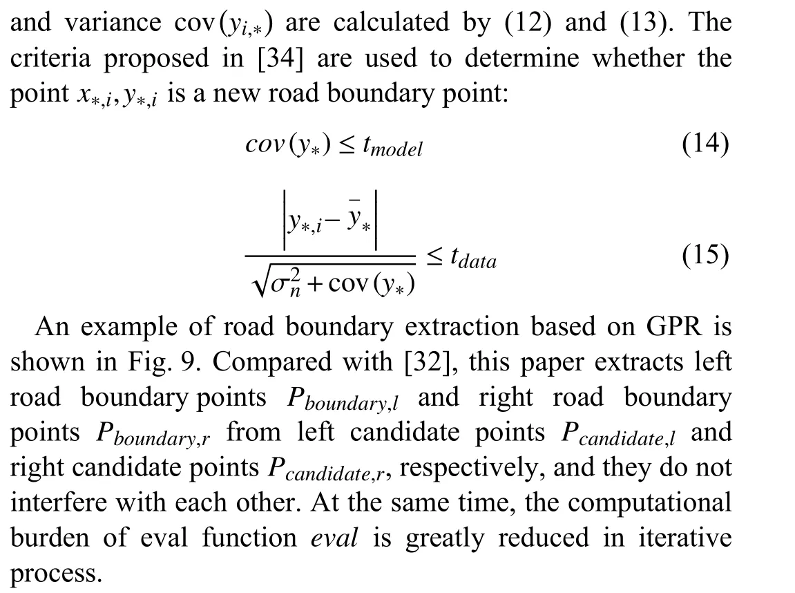
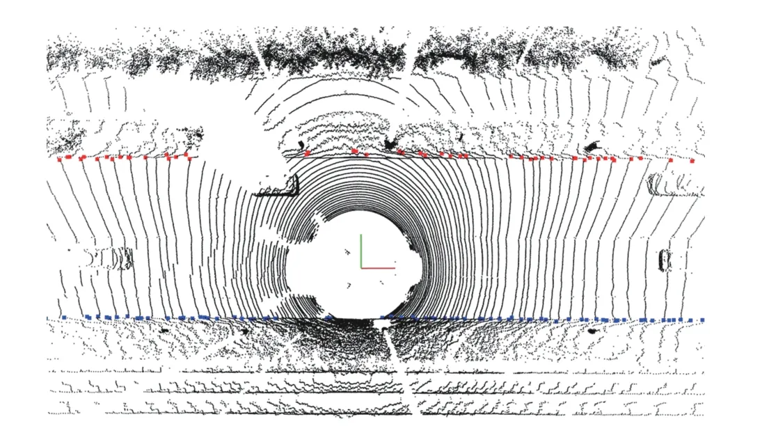
Fig. 9. Road boundary points extracted by GPR.
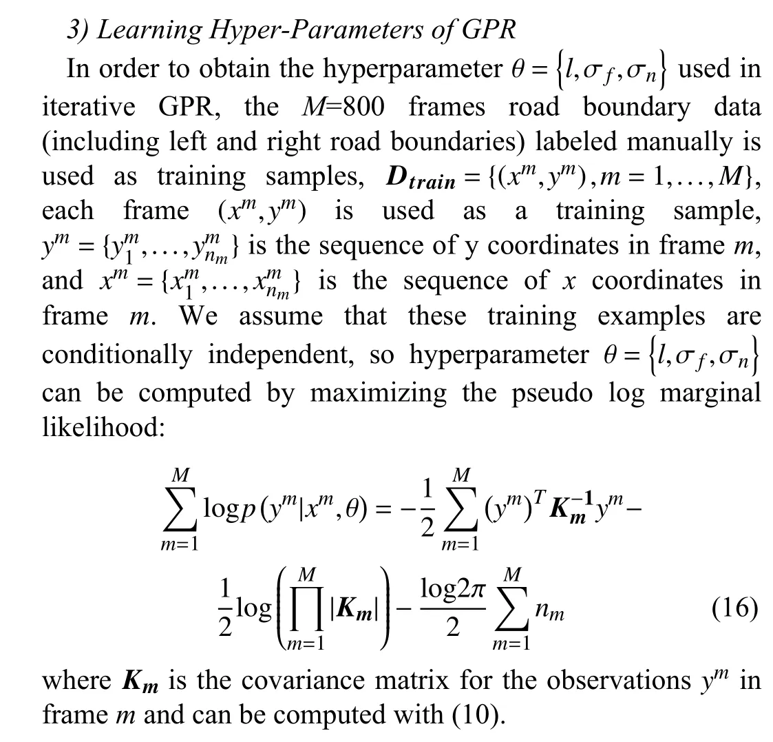
IV. EXPERIMENT EVALUATION AND ANALYSIS
To evaluate the proposed method in this paper, experiments were conducted on different road scenes. The experiments are divided into two parts. The first part is the qualitative experiment on the validity of the proposed method, and the second part is a quantitative experiment measuring accuracy and real-time performance. The KITTI Velodyne dataset [35]is used to evaluate the proposed method, which mainly covers urban and highway scenes. To demonstrate the effectiveness of our method on different road conditions, the proposed method is tested and evaluated on four typical road scenes(straight road, curved road, road with obstacles, and road with varying width). For each road scene, we manually labeled 500 frames for the road boundaries with the SemanticKITTI labeling tool [36]. The method is implemented by C++ and point cloud library (PCL) on Ubuntu 16.04.
In order to demonstrate the effectiveness of the proposed method, Zhang’s [27] and Sun’s [20] methods are employed for comparison. The values of parameters in our road boundary detection method are defined in Table II.

TABLE II PARAMETERS FOR OUR EXPERIMENTS
A. Qualitative Evaluation of Road Boundary Methods
For straight roads, as shown in Fig. 10, all three methods work well, and the results are similar because the road conditions are simple, and road boundaries are regular. Only spatial features and constraints can extract road boundary points well.
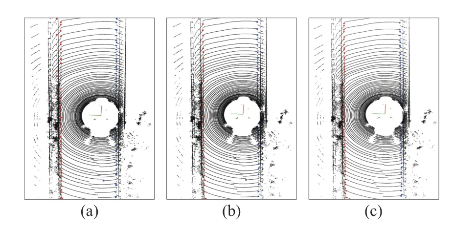
Fig. 10. The results of three methods on straight roads (left is in red, right is in blue). (a) Zhang. (b) Sun. (c) Proposed.
For a straight-curved road, as shown in Fig. 11, Zhang’s has some misclassified points, which shows the peak-finding method is not robust for the sparsity of point cloud. The proposed improved peak-finding method and Sun’s achieve accurate classification for road boundary points on curved roads.
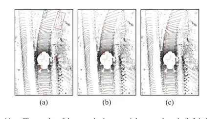
Fig. 11. The results of three methods on straight-curved roads (left is in red,right is in blue). In the red box are false points, and in the blue box are the points that have been misclassified. (a) Zhang. (b) Sun. (c) Proposed.
From Fig. 11 through Fig. 14, we can see that Zhang’s and Sun’s have false points caused by surrounding obstacles, such as vehicles inside roads, grass, shrubs, and railway tracks because they only remove false points based on spatial and geometric features. On the contrary, the proposed iterative GPR method can filter false points caused by obstacles. The qualitative evaluation experiments illustrate that the proposed method is accurate and robust for various road scenes and achieves better performance than other methods.
B. Quantitative Evaluation of Road Boundary Methods
1) Accuracy
The three different methods are also numerically evaluated on four typical road environments: straight roads, curved roads, roads with varying widths, and roads with obstacles.For these labeled frames, the labeled boundary points are projected onto a local grid map, which covers the detection region defined in Section III with the resolution of 0.15 m.Each cell of the grid map is classified into the left boundary,right boundary, or none; thus the ground truth of each cell is obtained. With the same method, the detection results of each cell can be obtained. When one cell is detected as the left boundary, and is also labeled as left boundary, we believe that this cell is detected correctly.

Fig. 12. The results of three methods on curved roads (left is in red, right is in blue). In the red box are false points, and in the blue box are the points that have been misclassified. (a) Zhang. (b) Sun. (c) Proposed.
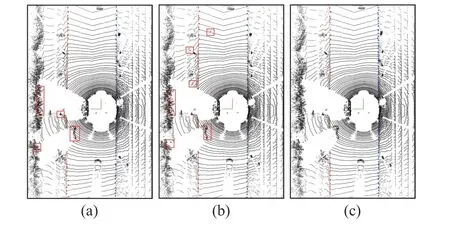
Fig. 13. The results of three methods on roads with obstacles (left is in red,right is in blue). In the red box are false points. (a) Zhang. (b) Sun. (c)Proposed.
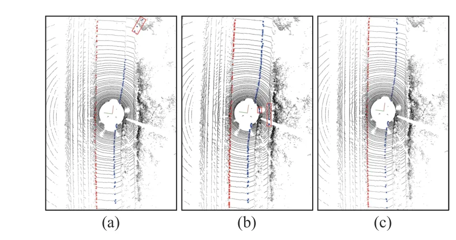
Fig. 14. The results of three methods on roads with varying widths (left is in red, right is in blue). In the red box are false points. (a) Zhang. (b) Sun. (c)Proposed.
To quantitatively evaluate our algorithm, three quantitative metrics in [37] and [38] are introduced for a comprehensive evaluation.
Precision, which denotes the proportion of cells detected correctly in all detected cells.

whereTPis the number of cells detected correctly, andFPis the number of cells detected incorrectly.
Recall, which denotes the proportion of the cells detected correctly in the labeled cells.

whereFNis the number of cells that are missed detections.
F1, which denotes the harmonic average ofPrecisionandRecall.

The quantitative evaluation and comparison are given in Table III. We can see that theRecallof our method is just slightly lower than Zhang’s and Sun’s because of the distance filter used in our method. Only one nearest point is preserved in the distance filter. However, because iterative GPR is used to model road boundaries and remove outliers, thePrecisionandF1of our method are the highest. It shows that the iterative GPR algorithm can effectively filter out false points and keep most boundary points. In addition, for the four different scenarios, theprecision,recall, andF1of the proposed method do not vary much, reflecting the robustness of the proposed algorithm.
In Zhang’s method [27], the bottom-layer beam model and the top-layer beam model were created based on the feature of the LiDAR sensor. Then, a rule-based peak-finding method was used to determine the road segmentation line. This method can achieve highPrecisionandRecallon straight roads. However,this method cannot handle outliers in distance functionδ(k)which may cause misclassification for boundary points. On the contrary, the improved peak-finding algorithm in this paper can easily deal with this problem and select the two most suitable dominant extremes. Besides, boundary points are directly extracted by three spatial features, and the obstacle occlusions were not considered. So, thePrecisionandF1of Zhang’s method are lower than the proposed method, especially on curved roads and those with obstacles.
In Sun’s method [20], first ground points are extracted by the polar-grid method, then road boundary points are directly detected based on a defined feature by searching along the predicted trajectory of vehicles. Because the trajectory was used to search boundary points, this method can correctly classify boundary points on various curved roads. However,the cumulative error of the predicted trajectory becomes larger as the scope of the prediction goes further, which would affect the accuracy of road boundaries. Similarly, the obstacle occlusions are also not considered, Sun’s method has higherRecalland significantly lowerPrecision. On the contrary,because iterative GPR has both powerful approximate and outlier rejection abilities, our method achieves significantly higherprecisionandF1with a small recall loss.
In conclusion, our proposed method can handle road boundary detection over various road scenes and achieves better performance. The other two methods achieve relatively poorer performance for obstacle occlusions and classification.
2) Runtime
We also evaluate the real-time performance of our method based on 1170 frames chosen from the KITTI dataset. Our experiments are performed on a 3.70 GHz Intel Core i7-8700 K processor with 16 GB of RAM. The runtime of our method is shown in Fig. 15. We can see that the running time of ourmethod is longer compared with Sun’s and Zhang’s, and the time spent on each frame varies greatly. The road boundaries of each frame are different, and the number of iterations of GPR varies, which results in violent fluctuations on time spent per frame. On the contrary, the methods of Sun and Zhang do not have false points filtering process. So, they have fewer and more consistent running times. However, our method can also perform with less than 100 ms per frame, with an average processing time of 70.5 ms. Because the scan period of LiDAR is 100 ms, real-time performance is achieved.

TABLE III QUALITATIVE EVALUATION RESULTS IN THE KITTI DATASET
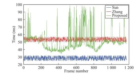
Fig. 15. The real-time performance comparison of three methods.
C. Failure Case
The method proposed in this paper is mainly aimed at road boundary detection in a structured non-congested traffic environment. The method achieved excellent performance under occluded, curved, and variable-width road conditions,as shown in Fig. 16. However, the proposed method achieves relatively poorer performance in heavy traffic environments and at complex intersections, as shown in Fig. 17. In Fig. 17(a),due to severe occlusion, our method incorrectly identified the side of the vehicles as the right road boundary.
V. CONCLUSIONS

Fig. 16. Successful cases of the proposed road boundary method. (a) Roads with obstacles. (b) Roads with varying widths. (c) Roads with large curvatures.

Fig. 17. Failure cases of the proposed road boundary method. (a) Roads with traffic congestion. (b) Roads with intersection. (c) Y-shape roads.
This paper presents an effective road boundary detection method with speed and accuracy tradeoff in structured environments. A multi-feature loose-threshold method is applied for feature points extraction. In order to classify feature points, road segmentation lines are determined based on the beam band model and improved peak-finding algorithm. The road segmentation line can be determined exactly under curved roads up to 70 m away. Then, the distance filter and RANSAC filter are applied to extract candidate points and seed points. Finally, an iterative GPR is proposed to filter out false points and extract boundary points. Based on seed points, the iterative GPR can remove false points caused by road users. Because iterative GPR is a nonparametric model, it can handle various road shapes well. Comprehensive experiment evaluations clearly demonstrate that our proposed method can obtain real-time performance and achieve better accuracy, especially on occluded and curved roads.
The method proposed in this paper is mainly aimed at road boundary detection in a structured non-congested traffic environment. In future works, we will focus on solving road boundary detection under traffic jams and complex intersections. In addition, we will simultaneously solve the problem of long-distance road boundary detection, which is necessary for high-speed driving.
杂志排行
IEEE/CAA Journal of Automatica Sinica的其它文章
- Distributed Asymptotic Consensus in Directed Networks of Nonaffine Systems With Nonvanishing Disturbance
- Finite-Time Fuzzy Sliding Mode Control for Nonlinear Descriptor Systems
- A Novel Rolling Bearing Vibration Impulsive Signals Detection Approach Based on Dictionary Learning
- Dual-Objective Mixed Integer Linear Program and Memetic Algorithm for an Industrial Group Scheduling Problem
- Output-Feedback Based Simplified Optimized Backstepping Control for Strict-Feedback Systems with Input and State Constraints
- Empirical Research on the Application of a Structure-Based Software Reliability Model
