Dual-Objective Mixed Integer Linear Program and Memetic Algorithm for an Industrial Group Scheduling Problem

Ziyan Zhao,, Shixin Liu,, MengChu Zhou,, and Abdullah Abusorrah, Senior

Abstract—Group scheduling problems have attracted much attention owing to their many practical applications. This work proposes a new bi-objective serial-batch group scheduling problem considering the constraints of sequence-dependent setup time, release time, and due time. It is originated from an important industrial process, i.e., wire rod and bar rolling process in steel production systems. Two objective functions, i.e., the number of late jobs and total setup time, are minimized. A mixed integer linear program is established to describe the problem. To obtain its Pareto solutions, we present a memetic algorithm that integrates a population-based nondominated sorting genetic algorithm II and two single-solution-based improvement methods,i.e., an insertion-based local search and an iterated greedy algorithm. The computational results on extensive industrial data with the scale of a one-week schedule show that the proposed algorithm has great performance in solving the concerned problem and outperforms its peers. Its high accuracy and efficiency imply its great potential to be applied to solve industrial-size group scheduling problems.

I. INTRODUCTION

AS an important branch of production scheduling problems, group scheduling problems (GSPs) have been increasingly concerned in recent years because of their extensive industrial applications [1]-[7]. In GSP, jobs to be scheduled are from several groups (or families). Those from a group have the same production requirements. In many industrial processes, jobs from a group are processed in serial batches [8], [9]. A so-called serial batch means that jobs within it have to be processed consecutively and thus its processing time equals the summation of the jobs’.

Two important classes of constraints, i.e., release time and due time, are commonly considered in scheduling problems[14]. The former is the time when a task becomes available for processing; while the latter is the time before which a task is expected to be completed. A scheduling problem considering the constraints of release time and sequence-dependent setup time, as well as an objective of minimizing makespan, is studied in [15], where a beam search algorithm is presented to solve it. A job is considered as a late one if it is completed later than its due time. The total number of late jobs (denoted asN～) is an important objective to be minimized in many scheduling problems [16]. A branch-and-bound method is designed in [17] to solve a single machine scheduling problem with periodic maintenance constraints and an objective of minimizingN～. A single machine scheduling problem with a time-dependent learning effect is studied in [18] to minimize～N, which is solved by a branch-and-bound method and two heuristics.

In some scheduling problems, a scheduler makes decisions based on multiple optimization objectives. Thus, many researchers focus on multi-objective scheduling problems[19]-[22]. Different from a single-objective one that is to find an optimal or near-optimal solution, a multi-objective one aims to find an optimal or near-optimal Pareto set (or Pareto front) containing its non-dominated solutions [19]. Multiobjective evolutionary algorithms (MOEAs) [23]-[28] are effective and popular to solve multi-objective optimization problems. Among them, a nondominated sorting genetic algorithm II (NSGA-II) [23] is a well-known and widely used one, which effectively solves some flexible job-shop scheduling problems [29] and flow-shop ones [30]. Recently,memetic algorithms which integrate population-based global search and individual-based local heuristic search show great performance in solving multi-objective optimization problems[31]-[33], and thus motivates this work.

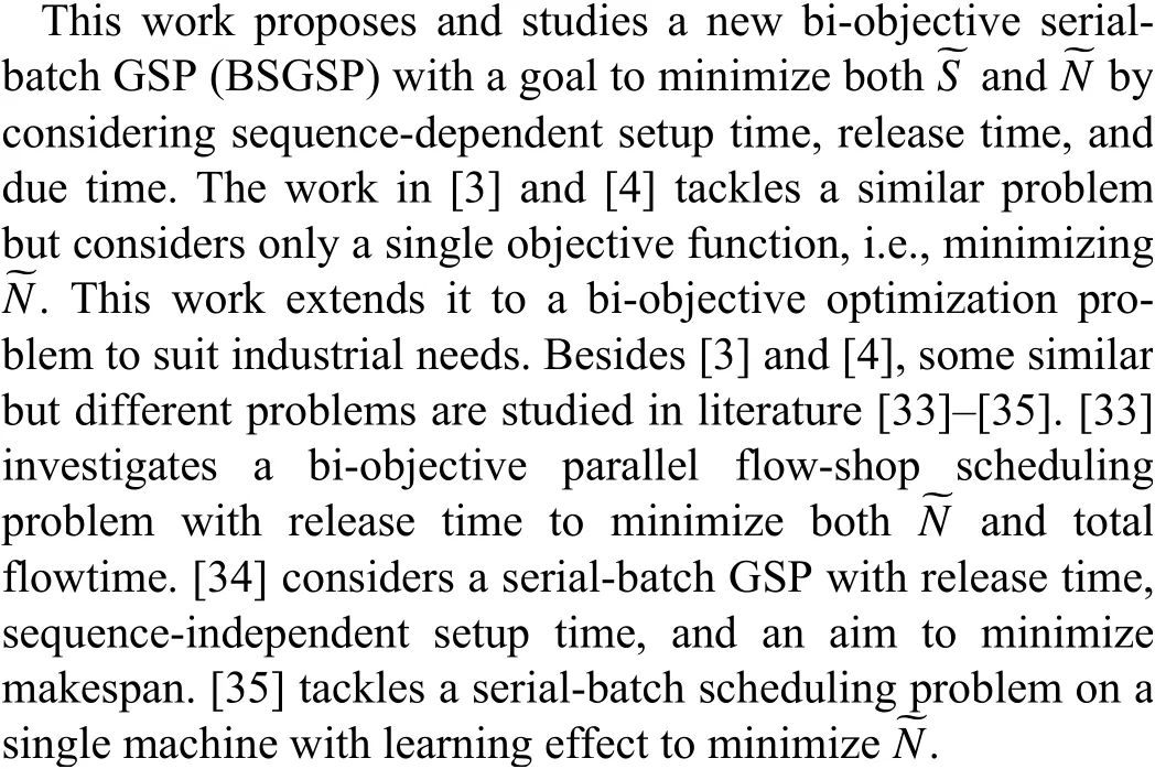
This work attempts to make the following contributions:

2) It establishes a mixed-integer linear program (MILP) to describe BSGSP in a rigorous way; and

3) It develops a new algorithm integrating NSGA-II and two individual-based improvement methods, i.e., an insertionbased local search and an iterated greedy algorithm, to solve BSGSP. In addition, this work compares the proposed algorithm with three competitive peers by extensive experiments to show its great performance and readiness for industrial applications.

Section II describes the concerned problem and formulates it into an MILP. A new algorithm is presented to solve the concerned problem in Section III. Experimental results are shown and analyzed in Section IV. Section V draws the conclusions and discusses some future research issues.

II. PROBLEM DESCRIPTION AND MODELING

A. Industrial Problem

A wire rod and bar rolling process plays a key role in steel production systems [3]. Steel ingots with short and thick shapes are processed into steel billets with long and thin shapes by going through a rolling mill as shown in Fig. 1. This work considers a single-machine scheduling problem on a rolling mill. Typically, a job in a rolling process is not just to deal with one steel ingot, but to continuously handle a set of steel ingots from a customer order, which have the same production and delivery requirements. A rolling mill has many positions to equip rolling stands as shown in Fig. 2 where 17 positions are available [36]. A rolling stand contains a pair of rollers in either parallel or vertical directions. The whole mechanical structure consisting of the equipped rolling stands is called a roll pass of a rolling mill. A roll pass can deal with the jobs with a range of specifications. Note that the rolling stands are not identical. Equipping different rolling stands on a position can lead to different size of steel billets. Apparently,the specification requirement of a job determines the roll pass of a rolling mill. If two jobs requiring different roll passes are processed consecutively, workers have to spend setup time in switching the equipped roll pass between them. In other words, some rolling stands need be equipped on or removed from the rolling mill. The setup time can be regarded as a linear function of the number of different rolling stands among the ones making up two roll passes [3].

Fig. 2. Schema of a rolling mill.

As a medium process of steel production systems, a rolling process has time limits from its upstream and downstream ones. A job in it can only be handled after being released by an upstream process and is expected to be completed before the due time required by a downstream process. A job becomes a late one if it is completed after its due time.According to industrial production rules, the jobs in a rolling process are assigned into some batches in advance. The ones in the same batch require the same roll pass and have to be processed continuously [3]. Realizing optimal scheduling for such an industrial process is very important for steel plants. In the scheduling problem, schedulers and practitioners must focus on minimizing two objective functions, i.e., the number of late jobs (N～ ) and total setup time (S～ ). ReducingS～ tends to continuously process the batches from the same family and thus may increaseN～; while reducingN～needs to process as many jobs as possible before their due time and thus may increase ～S, which results from frequent changes of machine states to satisfy production requirements. Hence, minimizing bothS～andN～causes a conflict.

B. Problem Transformation

To model and solve the above industrial problem, we transform it into a new single machine scheduling problem,i.e., a bi-objective serial-batch group scheduling problem(BSGSP). It has the following characteristics.Jjobs fromFfamilies are to be scheduled on a single machine. They have been arranged intoBserial non-preemptive batches in advance. The ones assigned into a batch are from the same family. Thus,J≥B≥F. There is no setup time between two consecutive jobs from the same batch. However, sequencedependent setup time is necessary between two consecutive batches if they are from different families. It is to change the machine states to satisfy different production requirements the two batches. The batches and jobs to be scheduled have their release time, processing time, and due time requirements.S～andN～are two objective functions to be minimized.

C. Mathematical Model

TABLE I NOTATIONS

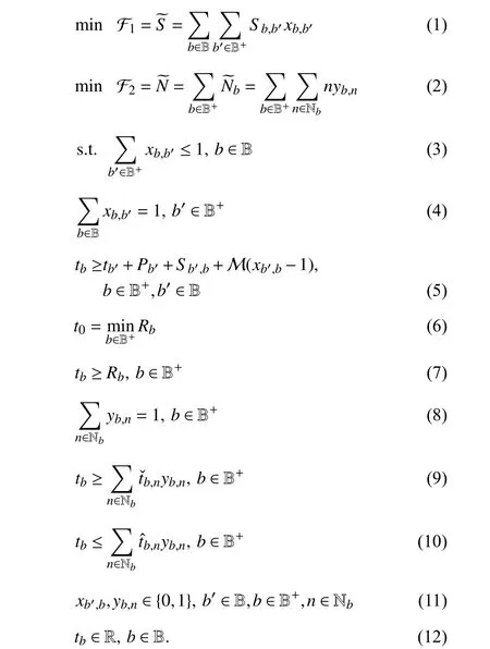
The objective functions in (1) and (2) minimizeS～andN～,respectively. Equations (3)-(7) together ensure a feasible batch sequence. Specifically, (3) means that there is at most one batch immediately after a batch. Only the last one is not followed by anyone. Equation (4) ensures that there is exactly one batch immediately before a batch to be scheduled. Note that the virtual batch as the first one is not restricted by it.Equation (5) ensures that at most one batch can be processed at a time, where M is a sufficiently large positive number. Ifxb,b′ =1, we rewrite (5) as

whereb∈B+andb′∈B. Otherwise, it is automatically relaxed. Equation (6) defines that the virtual batch starts from the earliest release time among all the batches to be scheduled.Equation (7) ensures that a batch is available only after its release time. Equations (8)-(10) together maptbtoN～b.Specifically, (8) ensures that a batch starts within exactly one time slot. Equations (9) and (10) provide its start time with lower and upper bounds. Equations (11) and (12) define the ranges of decision variables.

III. MEMETIC ALGORITHM

A. Encoding and Decoding

According to the problem description, we know that the concerned problem is to find batch sequences that satisfy the constraints and lead to non-dominated objective function values. Thus, we use a non-repetitive integer permutation of the elements from B to encode a batch sequence. For example,when scheduled three batches, a permutationπ=〈1,3,2〉means that batch 1 is the first one to be processed followed by batches 3 and 2.

B. Algorithm Design

We use each circle point in Fig. 3 to represent a solution of BSGSP. The hollow ones mean the solutions that are dominated by at least one of the others. The solid ones mean the solutions that constitute a Pareto front and are not dominated by the others. NSGA-II [23], [24] is a well-known MOEA, which is a population-based algorithm. However,when solving BSGSP with it, we find that the obtained Pareto front is far away from the ideal one. Thus, we design a novel memetic algorithm in Algorithm 1 by combining NSGA-II and two individual improvement methods, i.e., insertion based local search (ILS) and iterated greedy algorithm (IGA) [37] to solve BSGSP. Both ILS and IGA are single-solution-based algorithms that start from an initial solution and return a local optimal solution. For an easy description, we use NIMA to denote the proposed NSGA-II and Individual-improvementbased memetic algorithm.

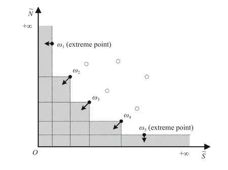
Fig. 3. Search space illustration of the proposed ILS.

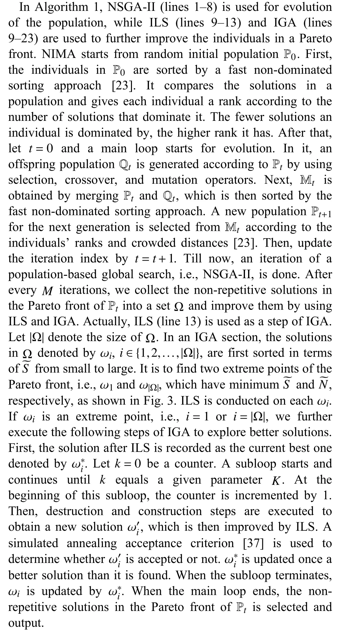
Algorithm 1: Outline of NIMA P0 M Input: A random initial population , a parameter to activate local search Output: A Pareto set Ω P0 1 Apply fast non-dominated sorting to to get its individuals’ranks;t ←0 2 ;not termination 3 while do Qt ←4 An offspring population whose individuals are generated by conducting crossover and mutation operations;Mt ←Pt ∪Qt 5 ;Mt 6 Apply fast non-dominated sorting to to get its

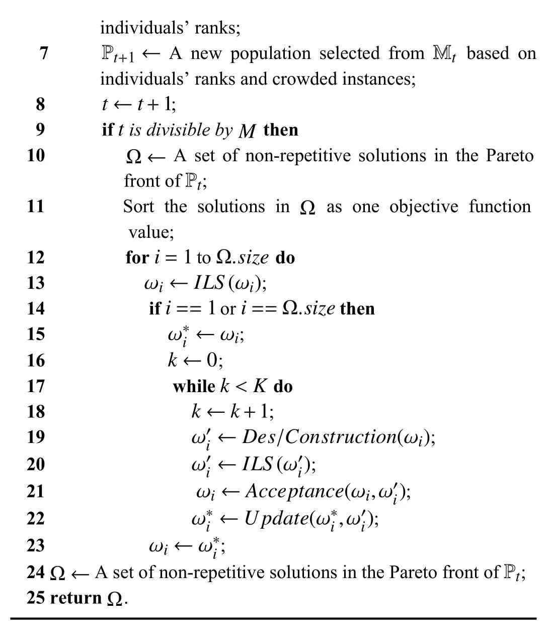
individuals’ ranks;Pt+1 ← Mt 7 A new population selected from based on individuals’ ranks and crowded instances;t ←t+1 8 ;t 9 if is divisible by then Ω ←Pt M 10 A set of non-repetitive solutions in the Pareto front of ;11 Sort the solutions in as one objective function Ω value;i=1 Ω.size 12 for to do ωi ←ILS(ωi)13 ;i==1 i==Ω.size 14 if or then ω*i ←ωi 15 ;k ←0 16 ;k ＜K 17 while do k ←k+1 18 ;ω′i ←Des/Construction(ωi)19 ;ω′i ←ILS(ω′i)20 ;ωi ←Acceptance(ωi,ω′i)21 ;ω*i ←Update(ω*i,ω′i)22 ;ωi ←ω*i 23 ;Ω ← Pt 24 A set of non-repetitive solutions in the Pareto front of ;25 return .Ω

C. Selection, Crossover and Mutation

In NIMA, three operators, i.e., binary tournament selection(BTS) [23], partially mapped crossover (PMX) [38], and reciprocal exchange mutation (REM) [33], are used. Their details are introduced as follows.

1) A BTS is to select a parent individual. It randomly selects two individuals in the current population and compare them with each other. If they have different ranks, the higher-rank one is selected. Otherwise, we randomly select one of them.

2) A PMX operator is used to generate two offspring individuals (denoted by O1 and O2) after selecting two parent individuals (denoted by P1 and P2) by twice runs of BTS. An example of its procedure is illustrated in Fig. 4. First, two cut points on parent individuals are randomly chosen. The portion between the cut points is inherited by the offspring individuals. Here, the one of P1 (resp. P2) is inherited by O2(resp. O1). Then, the mappings of the genes between the cut points are constructed. The rest genes of the offspring individuals are obtained by mapping the ones of the parent individuals to corresponding ones. Here, the genes mapped from the ones of P1 (resp. P2) are inherited by O1 (resp. O2).

3) An REM operator is to generate an offspring individual(O1) based on a parent one (P1). Fig. 5 shows its procedure,where two genes of the parent individual are selected and swapped to generate an offspring one.

D. Insertion-based Local Search

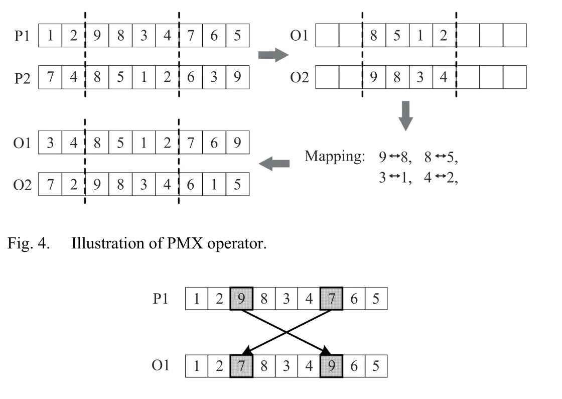
Fig. 5. Illustration of REM operator.

An ILS [37], [39] is used to further improve the solutions in the obtained Pareto front. Meanwhile, it is an important step of IGA. The shadows and arrows in Fig. 3 illustrate its search space. For a solution in the current Pareto front, we explore the space that dominates it. If it is an extreme point, we additionally explore the space that does not dominate it but leads to smaller single objective function value than it.Algorithm 2 shows its procedure that is conducted on each non-repetitive solution in a Pareto front. In it, the best solution π*is initialized by the input solution π. An iteration starts to randomly select a gene without repetition and remove it from π. Then, the best position is selected to reinsert it. When doing it, the removed position is initially marked as the best one followed by going through all the positions and comparing them with the marked one. Once a better position is found, it is marked as the best one. Let πMand πPbe two solutions obtained by inserting the removed gene into the marked position (denoted bym) and another one (denoted byp),respectively. According to different input solution π,pis considered as a better position thanmif it satisfies the following conditions:

1) For π=ω1, a) πPhas smallerS～than πM, or b) πPhas the sameS～as πMbut smallerN～than it.

2) For π=ω|Ω|, a) πPhas smallerN～than πM, or b) πPhas the sameN～as πMbut smallerS～than it.

3) For others, πPdominates πM.

If the best position is not the removed one, we consider that the solution π after reinsertion is better than π*, i.e., π ≺π*.Then, π*is updated by π. The search procedure terminates if π*is not updated in an iteration or 10 iterations are performed.

Algorithm 2: Insertion-based local search Input: A current solution π Output: A local optimal solution improve=true 1 ;π*iteration=0 2 ;π*=π 3 ;improve&iteration ＜10 4 while do improve= false 5 ;iteration ←iteration+1 6 ;i=1 B 7 for to do π 8 Select and remove a gene randomly from without repetition;π ←9 Insert the gene into the best position;π ≺π*10 if then π*=π 11 ;

improve=true 12 ;13 return .π*

E. Destruction and Construction

ILS provides a local optimal solution, which is broken out by destruction and construction steps of IGA as shown in Algorithm 3. In a destruction step, the batches fromIrandom families are removed from a solution π , whereIis a parameter to be adjusted. The removed ones constitute a subsequence called πDand the remaining ones are in a subsequence called πR. In a construction step, the batches in πDare reinserted into the best positions of πRone by one to construct a new solution. The so-called best position is defined depending on the input solution π.

2) If π=ω|Ω|, the best position means the one that leads to a subsequence (or sequence) with minimum makespan after insertion. Smaller ～Sis considered as a tie-breaker.

Note that we use makespan rather thanN～to evaluate a subsequence sinceN～of a subsequence can be significantly changed by subsequent insertions.

Algorithm 3: Destruction and construction π Input: A current solution π′Output: A new solution 1 Select families randomly;2 Remove the batches from the selected families;πD ←3 A subsequence consists of the removed batches;πR ←4 A subsequence consists of the remaining batches;i=1 πD.size 5 for to do π′← πDi πR 6 Insert into the best position of ;π′7 return .I

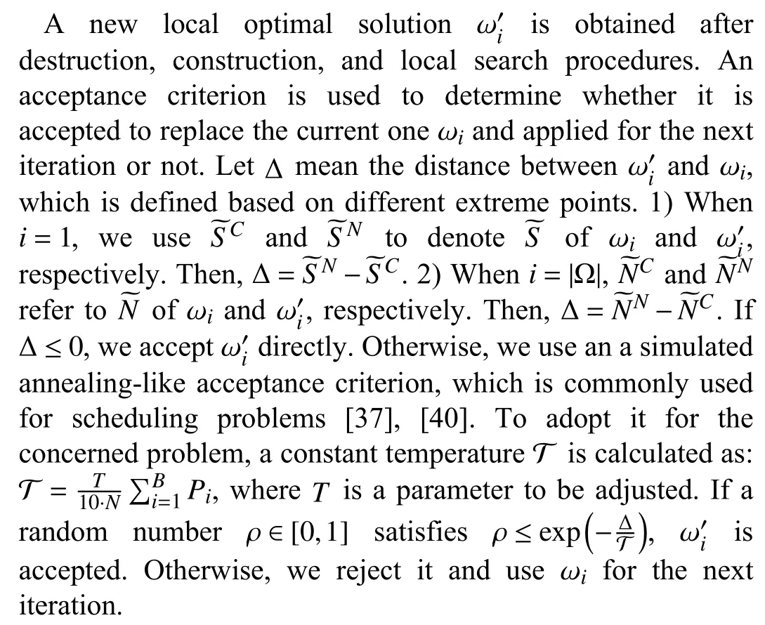
F. Acceptance Criterion

G. Computational Time Complexity

IV. EXPERIMENTAL RESULTS

A. Experimental Design

We use 14 400 experiments to test the proposed NIMA. The experiments are conducted on a dataset from a wire rod and bar rolling process [3]. The work in [3] uses the same industrial dataset to study a single-objective optimization problem while this work uses it to consider a bi-objective one.Nine groups of instances with differentBandJare used.Their scales range fromB=20 andJ=80 toB=40 andJ=240. The maximum scale is equivalent to one-week workload in a factory [3]. Each group contains twenty instances and thus 9 ×20=180 ones are solved in total.

To show the effectiveness of NIMA, we compare it with three MOEAs, i.e., NSGA-II [23], NSGA-III [26], and a recent peer denoted by NMMA, which is an NSGA-II and Mutation-local-search-based Memetic Algorithm [32]. For all the algorithms, they share the same population size, crossover and mutation rates, which are 100, 1 and 0.1, respectively.

The algorithms are all coded in C++ and run on a laptop computer with 32 GB of RAM and an Intel Core i7-8850H,2.60 GHz processor. When solving an instance, for a fair comparison, all the algorithms share the same termination criterion which is the limited running time when an NSGA-II takes for 8000 iterations. Table II demonstrates the average termination time for solving an instance with givenBandJ.To reduce the impact of the randomness on algorithm performance, we run each of them 20 times to solve an instance. The average solutions are summarized and compared with each other. Therefore, we perform180×4×20=14400 experiments in this work for algorithm comparisons.

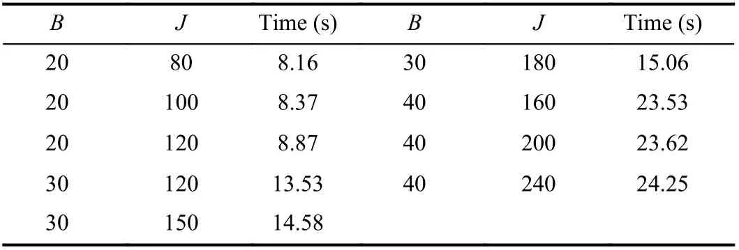
TABLE II TERMINATION CRITERION

B. Evaluation Metrics

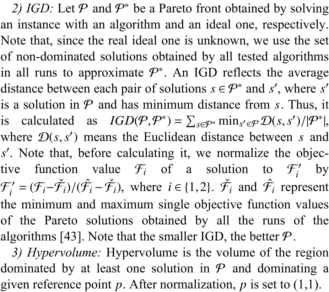
Three kinds of metrics, i.e., extreme points, inverted generational distance (IGD), and hypervolume, are used to evaluate the tested algorithms [42].

1) Extreme Points:Extreme points have the minimum single objective function values and thus are essential metrics to evaluate an algorithm. For many practical multi-objective scheduling problems, the solutions of the extreme points are important guides for practitioners.

C. Parameter Adjustment

Orthogonal experiments [43] are designed to adjust the four parameters of NIMA, i.e., 1)M: the number of iterations of NSGA-II before activating ILS and IGA; 2)K: the number of iterations of IGA for improving a Pareto solution; 3)I: the number of families to be removed in a destruction step; and 4)T: a temperature coefficient. For each of them, three candidates are given, i.e.,M∈{100,300,500},K∈{1,3,5},I∈{1,2,3} , andT∈{1,5,10}. NIMAs with nine parameter combinations (denoted by G1-G9) are used to solve ten instances withB=30 andJ=150. The average experimental results are shown in Table III. The parameters in G4 leading to the largest hypervolume are selected as the best combination and used for the following experiments. Note that we draw a box plot to show the hypervolume metrics of NIMA with different parameter combinations in Fig. 6. Itshows that different combinations lead to similar hypervolumes, i.e., NIMA is parameter-insensitive.

TABLE III PARAMETER ADJUSTMENT OF NIMA

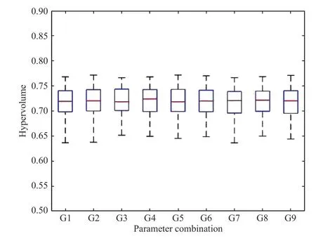
Fig. 6. Comparison of different parameter combinations.

D. Results and Comparisons

Tables IV and V compareS～andN～obtained by the four algorithms, denoted byS～aandN～a, wherea∈{i,ii,iii,iv}, i.e.,the extreme point comparisons. Note thatS～ is measured in hours. The optimal solution or near-optimal one ofN～ is denoted byN～*and given in [3], where CPLEX, i.e., a wellknown commercial optimization solver, is used to solve an MILP. The optimal solution of ～Sis denoted by ～S*and can be obtained by using CPLEX to solving an MILP consisting of(1), (3)-(7), and a redundant constraint as follows;

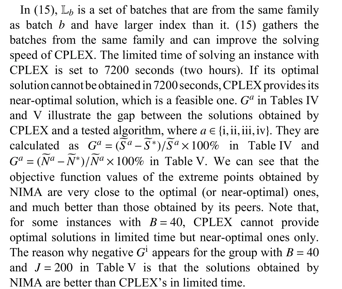
Table VI demonstrates the IGD comparisons of the Pareto fronts obtained by the tested algorithms. NIMA gets the smallest IGD followed by NSGA-III, and is much better than NSGA-II and NMMA. Especially as the scale of the problem increases, NIMA can solve the instances with small IGDs but its peers’ become larger and larger.

TABLE IV～S COMPARISON

TABLE V～N COMPARISON

TABLE VI IGD COMPARISON

In terms of hypervolume metric, our comparison is shown in Table VII, which indicates that NIMA has better performance than its peers. Similar to IGD, the hypervolumes of the compared algorithms get worse and worse as the problem scale increases, but NIMA keeps a great one.

In addition, we adoptt-test with 38 degrees of freedom at a 0.05 level of significance to show the performance comparison of NIMA and its peers. The results in Tables IVVII marked by using (+), (-), and (～) mean that NIMA is significantly better than, significantly worse than, andstatistically equivalent to its peers, respectively [44]. We can see that NIMA is significantly better than the compared algorithms for all groups of instances in terms of all evaluation metrics.

To clearly and intuitively illustrate the effectiveness of the proposed algorithm, in Fig. 7, we draw the final Pareto front obtained by NIMA and its peers when solving three randomly selected instances with different size, i.e., the ones with small(B=20 andJ=80) , medium (B=30 andJ=150), and large(B=40 andJ=240) scales. The so-called final Pareto frontof an algorithm consists of the non-dominated solutions after merging the Pareto solutions of 20 independent runs. For the small-scale instance a), Fig. 7(a) shows that the difference of the final Pareto fronts obtained by the four tested algorithms is not significant. However, as problem scale grows, in Figs. 7(b)and (c), the final Pareto fronts obtained by NIMA are clearly better than those of its peers.

Fig. 7. Final Pareto front comparison.

From the above comparisons, we can draw the conclusions that NIMA can well solve BSGSP and outperforms its peers.According to the termination criterion as shown in Table II,NIMA can solve the concerned problems with practical scales in very short time. Since the largest-scale instance withB=40 andJ=240 is equivalent to an actual scheduling problem in one week [3], which is a common scheduling period used in practice, NIMA has great potential to be applied to a factory.

V. CONCLUSIONS AND FUTURE WORK

This work tackles a new bi-objective serial-batch group scheduling problem with release time, due time, and sequence-dependent setup time. It arises from a practical industrial production system and aims to find a batch sequence to minimize both the number of late jobs and total setup time. A mixed integer linear program is formulated to describe it. Then, we design a novel memetic algorithm, based on hybrid NSGA-II, insertion-based local search, and iterated greedy algorithm, to solve it. Computational results of many experiments show the great effectiveness of the presented algorithm by comparing the extreme points obtained by it with the optimal or near-optimal solutions and comparing its performance with its three peers’. Its high solution accuracy and speed prove its great potential to be applied in practice.

As future research, we plan to extend the considered problem with real-world constraints, such as uncertain release time and processing time [35], [45]. The proposed algorithm can be problem-specifically modified to solve various similar problems [46]-[66].