An Ellipsoidal Set-Membership Approach to Distributed Joint State and Sensor Fault Estimation of Autonomous Ground Vehicles
2021-06-18EmanMousavinejadXiaohuaGeSeniorQingLongHanTengJoonLimandLjuboVlacicSenior
Eman Mousavinejad,, Xiaohua Ge, Senior, Qing-Long Han,,Teng Joon Lim,, and Ljubo Vlacic, Senior
Abstract—This paper is concerned with the problem of distributed joint state and sensor fault estimation for autonomous ground vehicles subject to unknown-but-bounded (UBB) external disturbance and measurement noise. In order to improve the estimation reliability and performance in cases of poor data collection and potential communication interruption, a multisensor network configuration is presented to cooperatively measure the vehicular yaw rate, and further compute local state and fault estimates. Toward this aim, an augmented descriptor vehicle model is first established, where the unknown sensor fault is modeled as an auxiliary state of the system model. Then, a new distributed ellipsoidal set-membership estimation approach is developed so as to construct an optimized bounding ellipsoidal set which guarantees to contain the vehicle’s true state and the sensor fault at each time step despite the existence of UBB disturbance and measurement noises. Furthermore, a convex optimization algorithm is put forward such that the gain matrix of each distributed estimator can be recursively obtained. Finally,simulation results are provided to validate the effectiveness of the proposed approach.
I. INTRODUCTION
RECENT advances in vehicle sensing and computing devices, intelligent driver-assistance systems, and wireless communication technologies during the last decade have considerably revitalized the development of autonomous ground vehicles (AGVs) [1] and autonomous surface vehicles[2]. As one of the components of intelligent transportation systems (ITS), AGVs with limited or no human intervention have been touted as a promising solution for improving vehicle safety and transportation efficiency, reducing traffic accidents, and providing an opportunity to conduct particular missions [3]. Moreover, advanced vehicular active safety technologies such as electronic stability program (ESP), active front steering (AFS), x-by-wire (XbW), and electric power steering (EPS) systems can effectively enhance passenger’s safety and driving comfort in AGVs [4]-[7].
The real-time values of yaw rate and sideslip angle are of significance in active vehicle safety technologies because they rely on this information for vehicle lateral risk assessment or adopt it as an input for a vehicle electric control unit. While the vehicle yaw rate can be directly measured by affordable gyroscopes, measurement of the vehicle sideslip angle is only possible through costly sensors such as two-antenna global positioning system (GPS) and optical sensors, which may not be economically viable in mass produced AGVs [8]. An alternative approach is thus needed to accurately estimate the sideslip angle with some relatively inexpensive on-board sensors already available in the vehicle.
Recently, there has been a surge of interest in the modelbased state estimation of vehicle sideslip angle. Up until now,several techniques have been proposed, which can be categorized into two main groups depending on the external disturbance and measurement noise models: 1) stochastic estimation methods (e.g., Kalman filtering and its variants)[9], [10] and 2) non-stochastic estimation methods (e.g.,H∞filtering and energy-to-peak filtering) [11]-[13]. It is wellacknowledged that the performance of stochastic estimation techniques rely heavily on accurate knowledge of particular statistical properties of disturbance/noise, such as mean and covariance of noise terms. However, when it comes to vehicular systems, the real driving conditions and vehicle environments can be complex and hence, the statistical properties of external disturbance and measurement noise are difficult to be accurately estimated. For example, as an external disturbance, the wind force acting on a vehicle is an irregular random sequence which is influenced by many factors including the windward side of the vehicle, the wind reference area, and the location of the center of pressure in the vehicle body [14]. Therefore, it is quite difficult to exactly know the statistical characteristics of the wind force disturbance in various driving conditions. For the measurement noise, consider a sensor measuring the vehicle yaw rate. At different driving conditions, the variance and standard deviation of the noise in a yaw rate sensor cannot be considered as constant since the measurement noise is not only caused by the physical or electronic characteristic of the sensor, but also by the vibration of vehicle chassis [15].However, the yaw rate sensor noise can be deterministically bounded since the friction coefficient of the road does not always let the vehicle’s tyres provide forces to support a high yaw rate [16]. In contrast to stochastic estimation techniques,the majority of non-stochastic estimation methods,particularlyH∞filtering, are based on an assumption of energy bounded disturbance/noise so as to find the worst-case solution to the vehicle state estimation problem [12].
Note that most of the existing estimation methods aim to determine asingle-vectorwith regard to the vehicle state such that the estimation error asymptotically converges to zero and thus, apoint-wiseestimation of the vehicle state is calculated.Such an estimation approach requires relatively higher sensor precision to steer the vehicle state estimation towards its true state. Besides, no hard bound on disturbance/noise signals means that there is no guarantee of some reliable confidence region enclosing entire distribution of the vehicle state,particularly when there exist external disturbance and measurement noise. This motivates the development of a surrogate technique called ellipsoidal set-membership estimation [17]. This method is aimed at computing a set bounded by an ellipsoid, which includes all possible state estimations while always enclosing the system’s true state based on the assumption that disturbance/noise signals are unknown-but-bounded (UBB) [18]. Under this assumption,the only stipulation is to acquire the knowledge of a hard bound on the disturbance/noise signal and hence, the need for gaininga prioriknowledge of the rigorous statistical characteristics of disturbance/noise is eliminated. Due to the exceptional power of the set-membership estimation technique in dealing with UBB disturbance/noise signals, such a method has been widely studied for various state estimation formulations in recent years [19]-[25].
Owing to the complexity of modern automated control and sensing systems, the unavoidable existence of faults in AGVs’physical components, i.e., actuators and sensors, jeopardizes vehicle stability and may even result in serious accidents.Examples of such failures are the blocking of an active steering actuator, unavoidable biases in a yaw rate sensor measurement due to uneven road or sensor circuit malfunctions, or a variation in its initial calibration factor due to a temperature drift error [26], [27]. The mitigation of faults requires some knowledge of their quantitative models. This can be fulfilled through implementing suitable fault estimation techniques. Over the last two decades, the problem of fault estimation has received considerable attention from different perspectives [23], [28]-[30]. In the context of vehicular systems, for example, an unknown-input proportional-multiintegral estimator is developed in [31] to estimate the vehicle state and the vehicle’s actuator and sensor faults in the existence of some disturbances. By treating the fault and disturbance as an unknown input, it is shown that their superposition can be estimated on condition that there only exists either a fault on the actuator or on the sensor. In [32], a proportional-derivative descriptor estimator is presented for a general discrete-time system to obtain the simultaneous estimates of the system state, actuator fault, sensor fault, and measurement noise. A vehicle dynamic system, which is equipped with the yaw rate and accelerometer sensors, is employed to demonstrate the effectiveness of their proposed method. Recently, a zonotopic-based set-membership fault estimation technique is developed in [23] for a discrete-time linear parameter-varying (LPV) system, where an augmented descriptor system model is presented and the zonotopic estimation interval size is recursively minimized in an effort to improve the estimation performance.
Stability performance of an AGV hinges on reliability and accuracy of sensor and/or estimator outputs and hence,sensors/estimators must guarantee the correctness and availability of the AGV’s state. However, in practice, the traditional single-sensor-based estimation technique of vehicle state may be unreliable due to sensor measurement contamination, sensor malfunction, or sensor aging.Therefore, it is of significance to construct a distributed estimation technique to estimate the vehicle state over a multisensor network. Such a network configuration is composed of a number of sensor nodes densely deployed in the vehicle.These nodes are linked together through a wired or wireless communication network. Therefore, the distributed estimation over a multi-sensor network has the key feature of utilizing the information collected from several sensors according to a prescribed interaction topology. (see [33]-[37] and the recent survey [38].) In this sense, the estimation accuracy and/or reliability may be improved through information sharing and exchanging among neighboring nodes. To the best of the authors’ knowledge, the problem of distributed setmembership joint estimation of vehicle state and sensor fault for AGVs has not been addressed, which motivates the current study.
In this paper, we develop a distributed set-membership estimation technique to jointly estimate an AGV’s lateral dynamical state, i.e., the yaw rate and sideslip angle, and sensor faults in the simultaneous presence of both UBB external disturbance and measurement noises. The main contributions are summarized as follows.
1) A joint distributed state and fault estimation configurationis established for an AGV subject to UBB external disturbance and measurement noises. To facilitate the process of sensor fault estimation, an augmented state including the vehicle yaw rate, sideslip angle, and sensor fault signal is formed to construct a descriptor model of the vehicle lateral dynamics in which longitudinal velocity is considered as a time-varying parameter.
2) A distributed set-membership estimation approachis developed so as to improve the reliability and resilience of the state estimates in the presence of sensor saturations and incomplete measurements. It is noteworthy that the proposed approach is capable of estimating each sensor’s fault, which may have different quantitative characteristics in practice.
3) A recursive and tractable convex estimation algorithmis derived for jointly estimating vehicle system state and sensor faults in real time. The algorithm aims to find a group of state estimation ellipsoids based on the incomplete and saturated measurement outputs received from individual sensors such that the vehicle’s true state and each sensor fault always reside in bounding ellipsoidal sets regardless of the UBB disturbance and noise. The proposed algorithm can also recursively determine the gain matrix sequences for each distributed estimator and shape matrix sequences for optimized ellipsoids.
The remainder of the paper is outlined as follows. Section II provides some preliminaries. Section III elaborates the vehicle lateral dynamics, the multi-sensor network configuration and the descriptor system model. Section IV presents the distributed set-membership estimators and also formulates the main problem. Section V derives the main results in terms of a distributed estimator design criterion and a recursive convex optimization algorithm. Section VI demonstrates the simulation results. Section VII draws a conclusion.
II. PRELIMINARIES
A. Notations

B. Sensor Interaction Topology
Let the sensor network haveNsensing nodes which are densely deployed in the vehicle according to a specific interaction topology represented by a weighted directed graph G=(V,E,A) , where V={1,2,...,N} denotes an index set of nodes, E ⊆V×V is an edge set of paired nodes, and A=[ai j]∈RN×Nis a weighted adjacency matrix whose elements are positive, i.e.,ai j>0 iff (i,j)∈E , andai j=0 otherwise. Ni={j∈V:(i,j)∈E} denotes the set of neighbors of nodei∈V plus the node itself.
C. Ellipsoid
Aboundedn-dimensionalellipsoidenclosinga realvector ζ∈Rnis denotedas E(c,P,ϱ)≜{ζ:(ζ-c)T P-1(ζ-c)≤ϱ},wherec∈Rnis thecenter,P∈Rn×nsatisfyingP=PT>0 is theshape matrix, and ϱ >0 is theradiusof the ellipsoid,which acts as a scaling parameter of the ellipsoid. The sum of squared semiaxes lengths of the ellipsoid is equivalent to the trace of its shape matrix, i.e., trace(P). Besides, thesizeof the ellipsoid is a function of the shape matrixP[39]. Hence,matrixPcan be time-varying so as to allow the ellipsoidal bounds to be adjusted over time.
Remark 1:Ann-dimensional ellipsoid E(c,P,ϱ) can be viewed as the image of an affine transformation of an ndimensional Euclideanuni t ball and hasyet anotherrepresentation as E ≜{ζ:ζ=c+ϱ12Qz,‖z‖≤1},whereQ∈Rn×mwith rank(Q)=m≤nandsatisfyingP=QQT>0is a lower triangular matrix with positive diagonal elements.
III. A MULTI-SENSOR DISTRIBUTED ESTIMATION CONFIGURATION
A. Vehicle Lateral Dynamics
A two-degree-freedom model [16] is adopted to describe the vehicle lateral dynamics, whose schematic is shown in Fig. 1 and vehicle’s parameters and their nominal values are described in Table I. Considering small sideslip angle β and front wheel steering angle δf, the lateral and yaw motions can be obtained as Fig. 1. Schematic of a two-degree-freedom lateral dynamics vehicle model.

TABLE I VEHICLE’S PARAMETER [40]

Parameter Symbol Value-Unit Vehicle's center of gravity CG -Mass of vehicle m 1832 kg Vehicle’s yaw moment of inertia Jz 2488 kg m2 Distance between CG and front axle lf 1.18 m Distance between CG and rear axle lr 1.77 m Front/Rear cornering stiffness cf/cr 96.240/107.180 kN/rad Front/Rear lateral tire force Fyf /Fyr N Front/Rear tire slip angle αf/αr rad

where ψ and ψ˙ are the vehicle yaw angle and yaw rate,respectively.
With the small front and rear tire slip angles, the total front and rear lateral forces are given by

where the tire slip angles can be expressed as

Substituting (2) and (3) into (1) yields the continuous-time state-space model of the vehicle lateral dynamics as

where the state vectorx(t)=[β(t)T,ψ˙(t)T]T, the control inputu(t)=δf(t)and

To capture the influence of external disturbances acting on the vehicle, such as wind force, road crown (sloping to one side of the road), and superelevation (banking turn), the external disturbancew(t) is incorporated in model (5) as

In this paper, we consider the UBB side wind force as an external disturbancew(t) which may influence the vehicle lateral dynamics. As discussed in [31], the corresponding external disturbance matrix can be represented asD′=[fw/mVx,lw fw/Jz]Twherelwis the distance of wind forceactionandfwisthewindforceandcanbeobtainedbyfw=Vw2AsρwwithVw,As,and ρwdenoting thewindvelocity perpendicular to the side surface of the vehicle, the side surface area of the vehicle, and the air density, respectively.
Note that, in practice, the vehicle longitudinal velocityVxis not always constant which results in time-varying system matrices in (5) asA′(t),B′(t), andD′(t). Hence, model (5) is a nonlinear system with respect to 1 /Vx(t) and 1 /Vx2(t). We next employ a Takagi-Sugeno (T-S) fuzzy modeling approach to deal with the nonlinear terms caused by the time-varying longitudinal velocity. To do this, the longitudinal velocity is assumed to be within the range [Vx,Vx], whereVxandVxare known lower bound and upper bound, respectively. In this case, one can obtain that
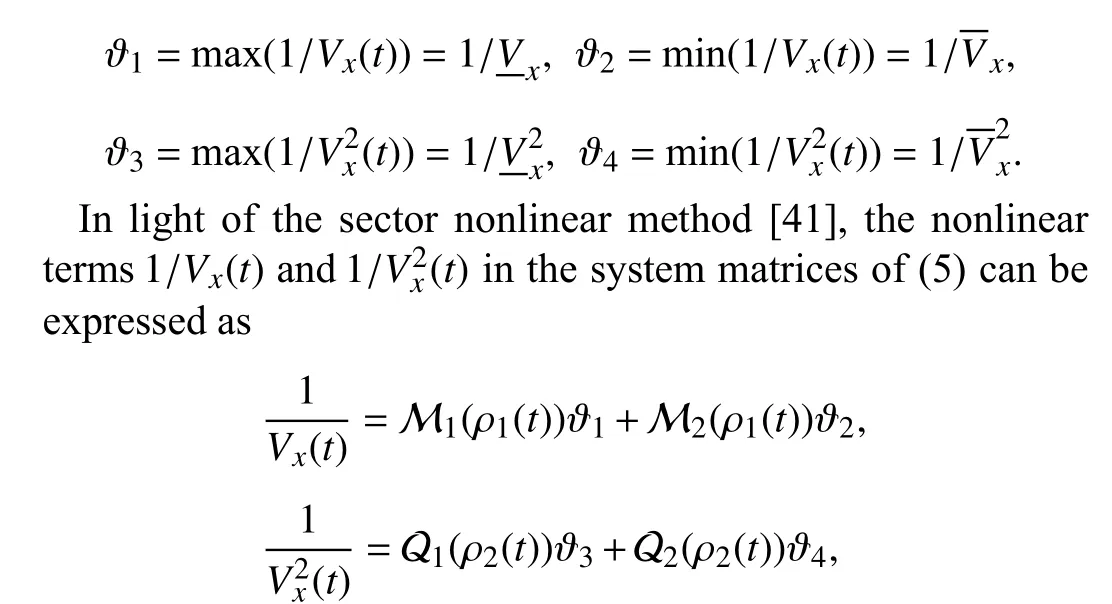
where ρ1(t)=1/Vx(t) and ρ2(t)=1/Vx2(t) represent the premise variables and M1(ρ1(t)), M2(ρ1(t)), Q1(ρ2(t)), and Q2(ρ2(t)) denote the membership functions withM1(ρ1(t))and Q1(ρ2(t)) stand for “High” longitudinal velocity, and M2(ρ1(t)) and Q2(ρ2(t)) stand for “Low” longitudinal velocity, respectively. More specifically, the membership functions satisfy

Then, T-S fuzzy expression of the vehicle lateral dynamics(5) can be given by the following rules
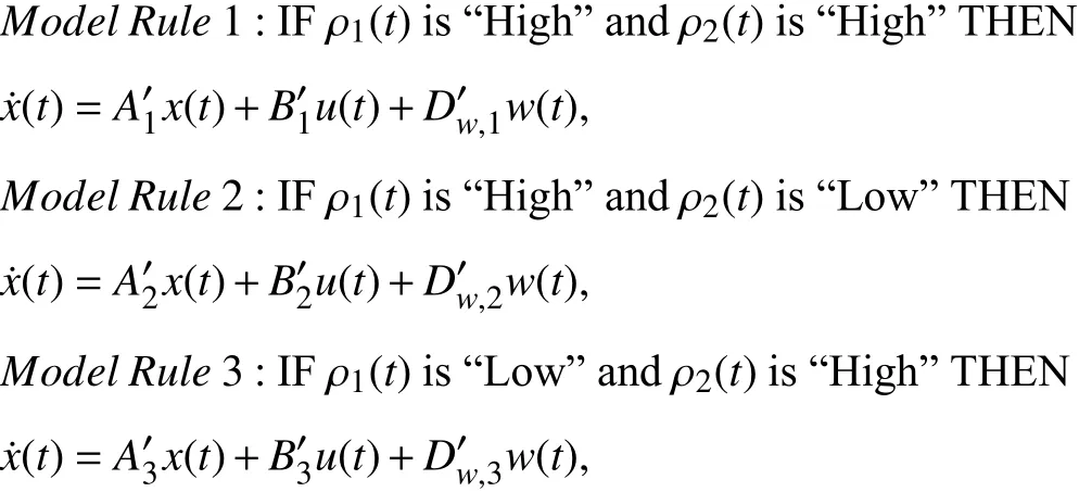
Model Rule4:IF ρ1(t)is“Low”and ρ2(t)is“Low”THEN
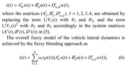
where the weighting functions αℓ(ρ(t)), ℓ =1,2,3,4 satisfy
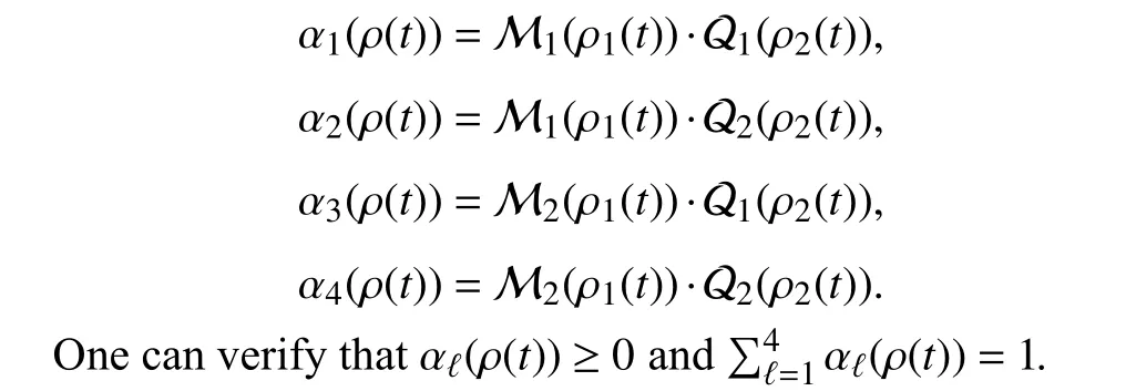
To facilitate the subsequent distributed set-membership estimator design, we further discretize the T-S fuzzy model of the vehicle lateral dynamics with a constant sampling period τs. To do so, the system matrices in (6) at the sampling period τscan be obtained by

anduk=u(tk) is sampled at the sampling instantstk=kτs. The UBB side wind force disturbance is assumed to be confined to the following ellipsoid:

Hence, the discretized T-S fuzzy model of the vehicle lateral dynamics can be expressed as

B. A Multi-Sensor Network Configuration
For eachi∈V , the measurement outputyi,k∈Rnyof sensoriin the presence of the sensor fault is given by

Remark 2:As discussed in [8], the yaw rate measurement is an appropriate choice for the sideslip angle estimation since the commercialized gyroscope can measure the yaw rate with no extra cost. Hence, the related element to the sideslip angle in matrixCican be set as zero, which indicates that sensorionly measures the yaw rate and thusny=1. In practice, the yaw rate sensors can be typically located either in the vehicle’s electric control unit, under the dashboard near the fuse box, or below the driver’s and/or the front passenger’s seats, mounted on the level floorboard in order to access the vehicle’s center of gravity [42].
C. A Descriptor System Model

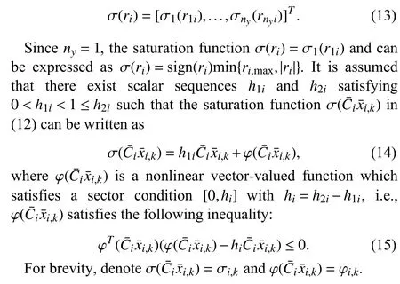
It is accepted that the measurement output of each sensor may be incomplete due to signal shading and channel fading[43], and/or network-induced data packet losses [44]. In addition, sensors may suffer from a common phenomenon known as “sensor saturation”, when measured signals lie outside the sensor’s dynamic range. Sensor saturation affects the estimation performance of the designed estimator, and may also cause instability of the system. Therefore, the incomplete measurement of sensoriin the presence of sensor saturation can be expressed as

The saturation function σ(·):Rny→Rnyfor sensoriin (12)is defined as
IV. DISTRIBUTED SET-MEMBERSHIP JOINT STATE AND FAULT ESTIMATION PROBLEM
It is our interest to develop a distributed set-membership estimation approach which includes a group of estimators computing some ellipsoidal sets of the augmented state estimation including vehicle state estimation and sensor fault estimation based on local measurement of neighboring yaw rate sensors. Each sensing nodei∈V consists of a processing unit, a buffer, and an estimator as depicted in Fig. 2. Suppose that the desired fuzzy estimatoriattached to sensorihas the following form
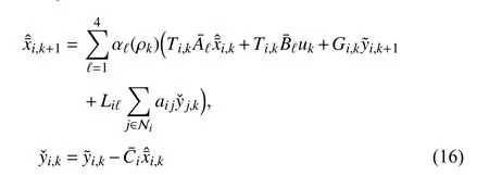
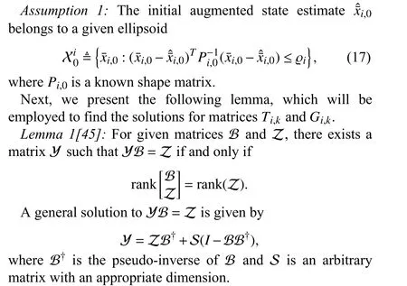
for allk∈N , wherei,k∈R(nx+nf)is the calculated estimate of the augmented stateat theith sensing node;i,kis the output of the processing uniti; the buffer in Fig. 2 stores data in a last-in-first-out manner and sends the one-step-behind data received from its own sensing node and the other nodes to estimatori;Ti,kandGi,kare the estimator matrix sequences tobedesigned;Liℓistheestimatori’sgainmatrix sequence to bedetermined;and,0is thegiveninitial condition,which satisfies the following assumption.
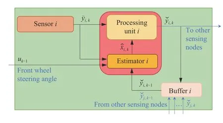
Fig. 2. Architecture of the ith sensing node in an AGV equipped with a multi-sensor network.
Remark 3:Since the descriptor system described by (11)and (12) satisfies that

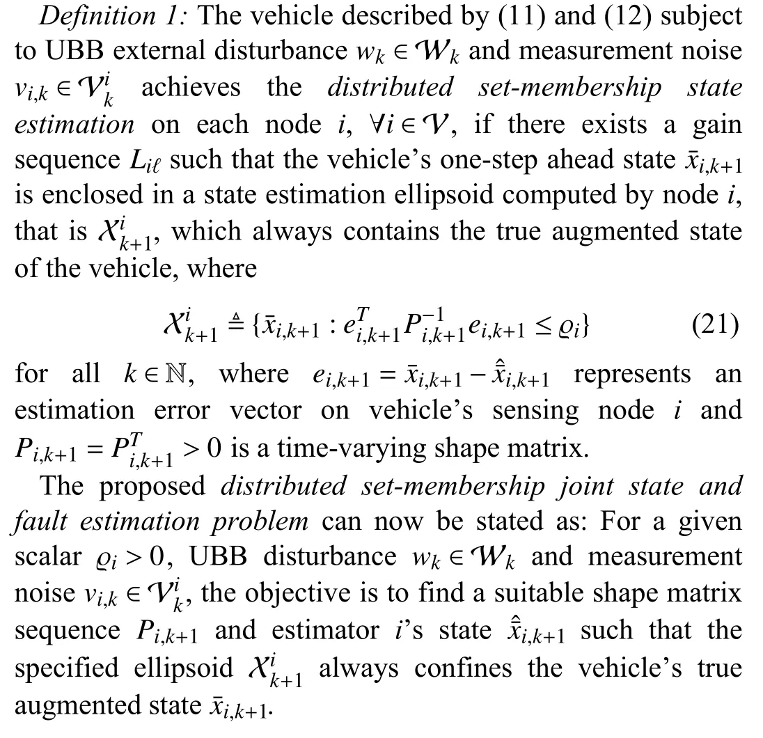
To proceed with the concerned distributed set-membership joint state and sensor fault estimation problem, we next introduce the following definition.
V. MAIN RESULTS
In this section, a theorem will be first established to provide a sufficient condition on the existence of the desired distributed estimators formulated in (16) such that (21) holds.Then, an algorithm will be presented so as to numerically solve the concerned distributed set-membership joint state and sensor fault estimation problem in a recursive manner.
To simplify subsequent analysis, we define the following notations:

A. Design Criterion
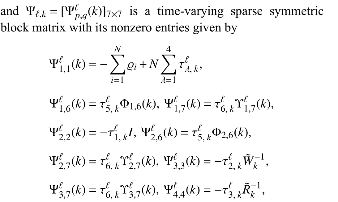
The following theorem outlines the sufficient condition on the existence of an optimized ellipsoidal estimate setat each sampling time on account of UBB external disturbance,UBB measurement noise, and incomplete and saturated measurement outputs received from individual sensors.



Remark 5:The interior-point algorithm usually has a polynomial-time complexity O(RM3), where R is the total row size of the main LMIs and M is the total number of scalar decision variables of the main LMI (22). Since R and M are dependent onnx,nu,ny,nw,nv, andnf, the computational complexity of the developed recursive algorithm depends polynomially on the dimensions of each sensing node’s parameter variables. Furthermore, the feasibility of Theorem 1 must be checked for each sensing nodei, ∀i∈V and thus, the total computation complexity of the main LMI (22) linearly depends on the number of sensing nodes.
B. Recursive Convex Optimization Algorithm
Based on (22), we next present a recursive distributed algorithm, i.e., Algorithm 1, that computes the real-time optimized augmented state estimation ellipsoids based on each sensor’s incomplete and saturated measurement output.Algorithm 1 also generates the gain matrix for estimatori(16)and determines its shape matrix sequencesPi,k+1.
VI. SIMULATION RESULTS AND CASE STUDIES
In this section, the developed distributed set-membership estimation approach is applied to investigate the joint state and sensor fault estimation problem of an AGV whose required parameters' values are given in Table. I. A network of six sensing nodes, i.e., V={1,2,...,6}, is deployed to cooperatively sense the vehicle yaw rate. The interaction topology of these nodes is demonstrated in Fig. 3, where the adjacency elementai jhas a binary value.

Fig. 3. Interaction topology of six sensing nodes measuring yaw rate.

Algorithm 1 Distributed Ellipsoidal State Estimation 1: Given initial conditions x¯0, xˆ¯i,0. For a given γ i,k ∈(0,1], a sensor i’s saturation setting, h1i and h2i , such that 0 <h1i <1 ≤h2i, and an arbitrary matrix S, calculate Ti,k and Gi,k by (19) and (20),respectively. Choose suitable W k, R i,k, and P i,0 such that (7), (10), and(17) hold. Calculate Mi,0 by Pi,0=Mi,0MiT,0 . Set k=0 , x¯i,k= x¯i,0,xˆ¯i,k= xˆ¯i,0, and M i,k=Mi,0. Let the simulation run for t seconds.2: Solve the OP (22) to obtain Pi,k+1 and Liℓ. Compute Mi,k+1 such that P i,k+1=Mi,k+1MiT,k+1.3: Compute the augmented state estimation xˆ¯i,k+1 by (16). Usexˆ¯i,k+1 ae s sti m th a e ti o cne nsteetr X ¯io,kf+1 t=h exˆ¯i,k e+s1t+i mϱi a12 tMi oin,k+1 e z li.l ipsoid Xi k+1 to calculate the 4: If k =t/τs go to Step 5; otherwise, set k =k+1, go to Step 2.5: Output matrix sequences {Pi,k+1} and {Liℓ}, fault vector estimate e x fˆˆiil s,,l kki p==s II¯o¯fx i xxˆ¯ˆ¯d ii,,a kk l,, sw ewth he{X er¯rei,e k + I ¯ x 1 I¯}=f.=[EInx[x 0i,t n0.fn×xn×xn, f I]n, f ]a n adn t d h e tahueg mv eehnitcelde s t sattaet e es e ti smt iamt i aotne

Furthermore, the corresponding weighting functions are depicted in Fig. 4.


Fig. 4. Vehicle longitudinal velocity, V x, front wheel steering angle δ f, and the weighting functions α ℓ(ρ(t)), ℓ =1,2,3,4.
The output of each yaw rate sensoriis subject to measurement noise asvi,k=cos(2πfcv(k-1)τs), wherefcv=idenoting the noise frequency. The measurement matrices are given byC1=[0, 3/25],C2=[0, 3/20],C3=[0, 9/50],C4=[0, 1/5],C5=[0, 4/25],C6=[0, 7/50], and the measurement noise matrices are set asDv,1=0.00873,Dv,2=0.01047,Dv,3=0.00542,Dv,4=0.00698,Dv,5=0.00785,Dv,6=0.0096.ChoosingWk=Ri,k=2 , one can easily check thatwkandvi,kbelong to the ellipsoidal sets defined in (7) and (10),respectively.
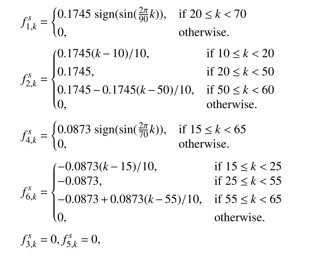
As discussed in [15], the common technical faults in a yaw rate sensor are sensor bias and drift, which refer to constant and slow-varying errors in the measurement signal,respectively. Such failures may be caused by sensor misalignment, variation in sensor temperature, sensor circuit malfunctions, and so on [27]. To model a constant and/or a slow-varying fault, a combination of step and ramp functions is considered to represent a fault signal in each yaw rate sensor as follows:fault matrices are chosen asDs,1=0.47,Ds,2=0.42,Ds,3=0.56,Ds,4=0.52,Ds,5=0.58, andDs,6=0.61.


The main objective is twofold: 1) To construct a bounding augmented state estimation ellipsoid for each sensing node so as to always enclose the vehicle true states, the yaw rate and the sideslip angle, and the sensor faults, at each time step, in the estimation ellipsoids of sensing nodes despite the UBB wind force disturbance and measurement noise; and 2) To perform a comparative analysis revealing the effects of the incomplete measurement and sensor saturation on the performance of the distributed joint state and sensor fault estimation process. In particular, we consider the following two different cases.
A. Neither Saturated nor Incomplete Measurement (NSNIM)Case


Fig. 5. Measurement output of sensor i (rad/s), ∀i ∈V, with fault and without fault yi.
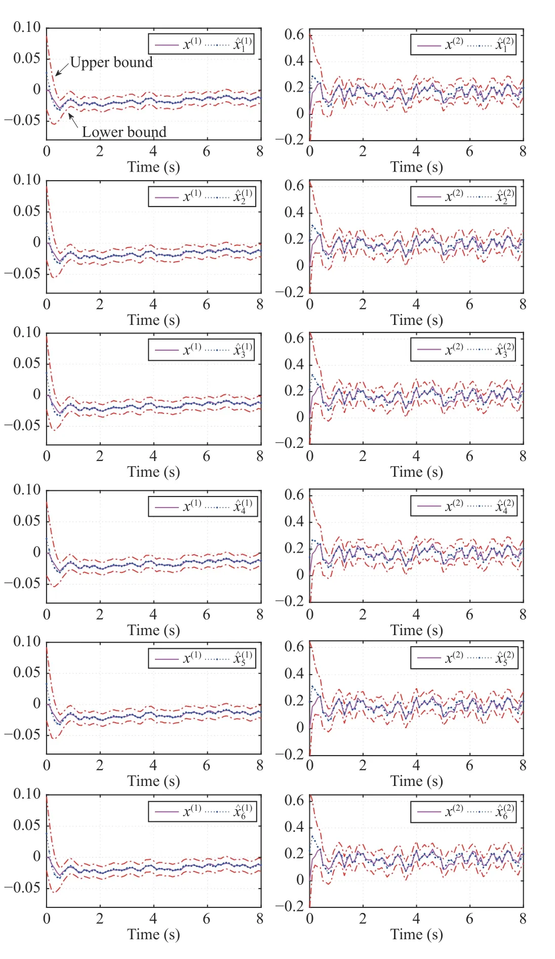
Fig. 6. True state of the vehicular sideslip angle x(1) (rad), yaw ratex(2)(rad/s), and their estimates , ), on sensing node i, ∀i ∈V as well as the state's upper and lower bounds.
In addition to the state estimation, Fig. 7 demonstrates that estimatoriis able to successfully provide the estimation of the fault on sensori. Also, as shown in this figure, the true value of each sensor fault is always confined in its confidence region limited with the upper bound and the lower bound computedbythe proposedset-membershipfault estimation technique through

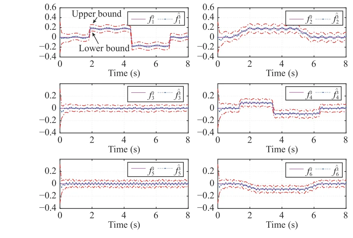
Fig. 7. Fault, fis (rad/s), its estimate, fˆis , on sensing node i, ∀i ∈V, the fault's upper and lower bounds.
B. Saturated and Incomplete Measurement (SAIM) Case
In this case, it is considered that the distributed estimatorimay receive incomplete and saturated measurement from its neighboring yaw rate sensors due to their physical constraints,technical limitation, and accidental data loss over the signal transmission. To model the incomplete measurement of sensori, the availability status of each sensor is chosen as γ1,k∈[0.72, 0.85], γ2,k∈[0.82, 0.95], γ3,k∈[0.76, 0.91],γ4,k∈[0.83, 0.98], γ5,k∈[0.78, 0.90], and γ6,k∈[0.87, 0.96].Also, the sensor saturation scalars are set ash1i=0.8 andh2i=1.1 ∀i∈V, and the maximum saturation levels are chosen asr1,max=0.08,r2,max=0.07,r3,max=0.035,r4,max=0.06,r5,max=0.03, andr6,max=0.025.
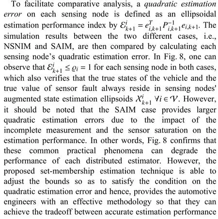
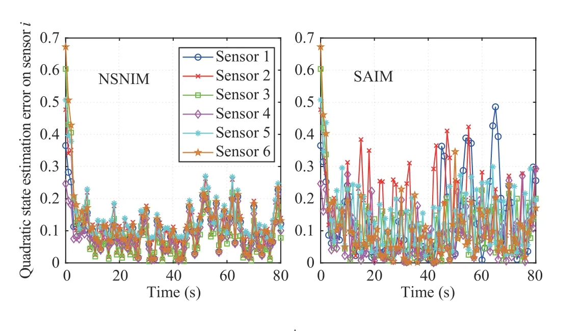
Fig. 8. Quadratic estimation error Eik+1 on sensing node i, ∀i ∈V in different cases of the NSNIM and the SAIM.

VII. CONCLUSION
The distributed set-membership joint state and sensor fault estimation problem over a multiple yaw rate sensor network configuration has been addressed for an AVG whose dynamics are under the influence of UBB external disturbance and measurement noise. Due to physical constraints, technical and communication limitations in real-world application of yaw rate sensors, it has been considered that each distributed estimator may suffer from sensor saturation and incomplete measurement signals. Distributed set-membership estimators have been constructed to estimate the vehicle yaw rate,sideslip angle, and each sensor’s fault. The design criterion for computing the desired estimators under varying longitudinal velocity consideration has been developed to guarantee that each estimator can provide a bounding ellipsoidal estimation of the vehicle’s true state and its sensor fault. To find optimized ellipsoids, a recursive convex optimization algorithm has been developed. Finally, comparative simulation results have been provided to demonstrate the effectiveness of the proposed results. As possible future research, how to develop an event-triggered distributed state and fault estimation approach for in-vehicle networked AGVs subject to limited resources is an interesting problem. Another potential research issue is to incorporate both sensor and actuator faults and further initiate an effective distributed fault detection and isolation approach for AGVs.
杂志排行
IEEE/CAA Journal of Automatica Sinica的其它文章
- Speed and Accuracy Tradeoff for LiDAR Data Based Road Boundary Detection
- Distributed Asymptotic Consensus in Directed Networks of Nonaffine Systems With Nonvanishing Disturbance
- Finite-Time Fuzzy Sliding Mode Control for Nonlinear Descriptor Systems
- A Novel Rolling Bearing Vibration Impulsive Signals Detection Approach Based on Dictionary Learning
- Dual-Objective Mixed Integer Linear Program and Memetic Algorithm for an Industrial Group Scheduling Problem
- Output-Feedback Based Simplified Optimized Backstepping Control for Strict-Feedback Systems with Input and State Constraints
