Deep Learning in Sheet Metal Bending With a Novel Theory-Guided Deep Neural Network
2021-04-16ShimingLiuYifanXiaZhushengShiHuiYuSeniorMemberIEEEZhiqiangLiandJianguoLin
Shiming Liu, Yifan Xia, Zhusheng Shi, Hui Yu, Senior Member, IEEE, Zhiqiang Li, and Jianguo Lin
Abstract—Sheet metal forming technologies have been intensively studied for decades to meet the increasing demand for lightweight metal components. To surmount the springback occurring in sheet metal forming processes, numerous studies have been performed to develop compensation methods.However, for most existing methods, the development cycle is still considerably time-consumptive and demands high computational or capital cost. In this paper, a novel theory-guided regularization method for training of deep neural networks (DNNs), implanted in a learning system, is introduced to learn the intrinsic relationship between the workpiece shape after springback and the required process parameter, e.g., loading stroke, in sheet metal bending processes. By directly bridging the workpiece shape to the process parameter, issues concerning springback in the process design would be circumvented. The novel regularization method utilizes the well-recognized theories in material mechanics, Swift’s law, by penalizing divergence from this law throughout the network training process. The regularization is implemented by a multi-task learning network architecture, with the learning of extra tasks regularized during training. The stress-strain curve describing the material properties and the prior knowledge used to guide learning are stored in the database and the knowledge base, respectively. One can obtain the predicted loading stroke for a new workpiece shape by importing the target geometry through the user interface. In this research, the neural models were found to outperform a traditional machine learning model, support vector regression model, in experiments with different amount of training data. Through a series of studies with varying conditions of training data structure and amount, workpiece material and applied bending processes, the theory-guided DNN has been shown to achieve superior generalization and learning consistency than the data-driven DNNs, especially when only scarce and scattered experiment data are available for training which is often the case in practice. The theory-guided DNN could also be applicable to other sheet metal forming processes. It provides an alternative method for compensating springback with significantly shorter development cycle and less capital cost and computational requirement than traditional compensation methods in sheet metal forming industry.
I. INTRODUCTION
SHEET metal forming has been employed in industry for centuries. Among different forming techniques, sheet bending and stamping are most widely used in sheet metal forming industry [1]. These techniques have been continually developed for over a century, especially in the last couple of decades, to meet the increasing demand for lightweight metal components with high strength to reduce weight and increase fuel efficiency in the automobile and aviation industries, due to the stringent emission control. However, subject to its high yield strength-to-elastic modulus ratio, high strength aluminum alloys and steels are predisposed to notably large springback. As a consequence, the manufacturing accuracy of conventional metal forming techniques would suffer. To address this issue, vast research on estimating the springback behavior in different sheet metal forming processes has been conducted experimentally and numerically [2]-[4].
To surmount the springback in sheet metal forming process,most of the current research focuses on developing compensation methods in numerical simulations or experiments [5],[6]. With finite element (FE) simulations, Lingbeek et al. [7]developed the smooth displacement adjustment (SDA) method and the surface controlled overbending (SCO) method to optimize the tool shape for a deep drawing process to increase the geometry accuracy of the product after springback. Lin et al. [8] developed a novel advanced forming method, hot form quench (HFQ®), for forming complex-shaped highstrength aluminum alloy sheets, which integrates hot stamping process with heat treatment and improves geometrical accuracy by minimizing springback. Wang et al. [9]developed a three-dimensional (3D) scanning method to replace the traditional special fixture for inspecting the part during the stamping of a rear reinforcement plate of a door panel, which was stated to increase the qualified rate of the product to a new peak. In creep age forming (CAF), Li et al.[10] proposed a one-step springback compensation method for singly curved products and an accelerated method for CAF tool design with reference to the springback compensation curves, which are established based on the numerical solution of springback behavior of CAF process. The effectiveness of the two methods was demonstrated by CAF experimental tests. Although springback occurring in different sheet metal forming processes has been significantly alleviated by the increasing amount of research in this area, the development cycle is still considerably time-consumptive and demands high computational or capital cost. In this context, the impressive prediction capability and low temporal cost of machine learning technology has attracted researchers to harness this novel artificial intelligence (AI) technology in sheet metal forming industry.
Over the last two decades, machine learning technology has been vastly applied to various manufacturing processes, such as metal forming [11], semiconductor [12] and nanomaterials manufacturing [13]. In sheet metal forming industry,supervised learning technology, compared to unsupervised learning [14] and reinforcement learning [15], is most prevailing. The research focus of supervised learning in sheet metal forming processes mainly resides in classification and regression. Traditional supervised learning algorithm includes support vector machines (SVM), decision tree, Naive Bayes classifier and K-nearest neighbors (KNN) algorithm [16],[17]. Liu et al. [18] used SVM to predict the springback of a micro W-bending process, and the SVM was demonstrated to have high prediction accuracy and generalization performance by comparing its prediction with experimental results. Dib et al. [17] compared the performance of several machine learning (ML) algorithms (multilayer perceptron, random forest, decision tree, naive Bayes, SVM, KNN and logistic regression) in predicting springback and maximum thinning in a U-channel and square cup forming processes. Among these models, multilayer perceptron was reported to be the best in identifying the springback, with slightly higher score than SVM. Apart from bending, Abdessalem et al. [19] compared the performance of a quadratic response surface method(RSM) and two least square support vector regression models(SVRs), with polynomial kernel (PL-K) and radial basis function kernel (RBF-K), in predicting a limit state function(LSF) to determine the best surrogate model used in a probabilistic approach for the structure optimization of hydroformed sheet metals. It was found that both SVRs outperforms the RSM in learning the nonlinearity of the LSF.
Neural network learning subsumes shallow and deep learning, which are commonly distinguished by the depth of learning and the depth of networks. To date, research on shallow learning dominates the development of machine learning in sheet metal forming [20]. For example, Narayanasamy et al. [21] compared the performance of a multi linear regression model and a four-layer artificial neural network(ANN) in predicting the springback angle of an air bending process, from which the ANN exhibited higher prediction accuracy than the regression model. Guo et al. [22] developed a combination of error back propagation neural network and spline function (BPNN-Spline) to predict the springback angle in a V-die bending process, in which the BPNN took sheet metal thickness, punch radius, die radius and a material indication parameter as inputs. The proposed BPNN-Spline model was demonstrated to outperform the traditional ANN in predicting the bending angles at different punch displacements. Viswanathan et al. [23] implemented a threelayer neural network to predict the stepped binder force trajectory at different punch displacement, thus realizing the control of springback in a plane strain channel forming process. Apart from the prediction of springback or forming parameters, shallow learning has also been used to substitute or reinforce the constitutive model for metallic material[24]-[26]. A three-layer neural network was developed by Jenab et al. [25] to predict the rheological behavior of AA5182-O sheet. Without the limitations of the mathematical function, the neural network was reported to outperform two phenomenological models, Johnson-Cook (JC) and Khan-Huang-Liang (KHL) models, in predicting the anisotropic rate-dependent behavior of AA5182-O. Li et al. [26]developed a machine-learning based JC plasticity model to capture the non-monotonic effect of the temperature and strain rate on the hardening response for DP800 steel. By combining shallow neural network and JC model, it was found that all experimental data can be described with high accuracy. In addition to using human designed features as the input to the neural network like above, Hartmann et al. [27] devised a four-layer network to predict the optimal tool path, by learning a processed form of desired workpiece geometry, for the production of sheet metals in an incremental sheet metal free-forming process. However, special attention had to be paid to the design of input and output to obtain good learning efficiency. It was claimed that, in order to cover the component spectrum, the cardinality of the training set needed to be significantly increased.
Unlike numerous studies in shallow learning, limited research has applied deep learning technology to sheet metal forming thus far. Since the great success of deep convolutional neural networks (CNNs) in learning and extracting physical features or even representations of data with multiple levels of abstraction from raw image-based inputs [28], [29], deep learning has brought breakthroughs in computer vision and image/speech/audio processing [30]-[32].Reaping the benefits from the notable advancements in computer science technology during the last two decades,deep learning has just revealed its extraordinary learning capability in discovering the latent pattern and regularities in a given data domain. With deep learning, instead of designing hand-crafted features as the input, the workpiece geometry information is fed into the network to achieve end-to-end learning and reduce the potential bias introduced in the design of input representation. It was believed to outperform shallow neural network learning and traditional machine learning techniques, such as KNN algorithm, when handling AI-level tasks with high data dimensions and complex functions [33].Consequently, researchers in sheet metal forming industry start resorting to deep neural network (DNN), which is an approximation model used in deep learning and consisting of relatively deep layers of neurons, for high-level learning or optimization. With deep learning, Hamouche et al. [34]demonstrated that a deep CNN can replace the traditional rulebased implementations in classification and selection of sheet forming processes for its higher accuracy rates. Jaremenko et al. [14] developed a CNN to determine the forming limit curve by learning and clustering the common patterns existing in sheet metal geometries before defects occur. DNNs have also been applied for the manufacturability prediction of sheet metals [35] and utilized as a surrogate model (or meta-model)[36], [37]. It was seen that deep learning technology was mostly applied to classification problems in sheet metal forming processes. However, most optimization problems in engineering involves parametric regression.
Yet, overfitting is a challenge in pure data-driven deep learning research, which frequently occurs when only scarce data are available or with improper training data structures.Besides, the inferior interpretability of the normal DNN has caused confidence shrinkage in its predictions, which confers it a title of “black box”. Acquiring massive experimental data in practice is also prohibitively expensive. Consequently,physics-informed neural network (PINN) was developed to prevent overfitting problems and alleviate the low interpretability issue by respecting prior expertise and guiding the learning process with governing equations in relevant theories. The most prevailing form of physics-informed deep learning is the physics-informed data assimilation regression with physics-informed regularization method. In this method,one or several governing equations in the research area,normally nonlinear partial differential equations (PDE), are used and converted to one or several physics-informed regularization term in the objective function. In [38]-[41],PINNs were used to predict numerical solutions of governing equations in computational fluid dynamics (CFD). It was reported to outperform pure-data driven DNNs with less training data. Besides of guiding deep learning with known governing PDEs, Tartakovsky et al. [38] used PINN to predict the unknown state-dependent coefficient in a nonlinear diffusion equation. Yao et al. [42] developed an FEA (finite element analysis)-Net which embeds the governing equation used in finite element analysis into the DNN design and consists of an FEA convolution network and an inference network, to predict FE simulation results for some simplified problems. These studies have shown the superiority of PINN over pure data-driven DNNs in generalization accuracy and demand of training data.
However, no PDE-like governing equations can be used to delineate the main physical features in most Lagrangianmechanics-like practical engineering problems with changing coordinates, especially when macro-scale parameters are of interests. To the authors’ knowledge, no attempt has been so far reported that utilizes a data-driven or theory-guided DNN(TG-DNN) in sheet metal forming industry for high-level optimization. The aim of the research is to fill in this gap.Thus, in this paper, two DNNs trained by pure training data or a novel theory-guided regularization method were developed for a learning system, named intelligent sheet metal forming system (ISMFS), and evaluated by applying them to sheet metal bending processes. By learning the intrinsic relationship between the workpiece shape after springback and the loading stroke, the springback could be compensated. The TG-DNN exploits a well-recognized theory in material mechanics,named Swift’s law, as the substitute for the PDE governing equations to regularize the network learning. Instead of regularizing the prediction of outputs of interests, the TGDNN incorporates multi-task learning configurations and improves the network generalization by regularizing the learning of extra tasks. With this method, the weights/biases distribution of the network would be potentially altered in a way that also facilitates the learning of the primary task,which has been corroborated in results obtained from a series of comprehensive numerical experiments in this research. A support vector regression model was also trained in this research, whose predictions were used as the baseline of learning results. The results in this research show that both data-driven and TG-DNN outperforms the SVR at the test phase. The TG-DNN can preserve high learning capability when only scarce training data are available, while the generalization accuracy of pure data-driven DNN has seen sufferings.
The contributions of this paper include: 1) filling the gap of forming process parameter prediction with deep learning in sheet metal forming industry; 2) proposing a novel theoryguided deep learning method which outperforms both traditional machine learning and data-driven deep learning methods in the prediction of non-linear behavior in sheet metal bending processes, when only scarce and scattered data are available; 3) improving the interpretability of the traditional neural model applied to metal forming industry; 4)providing an alternative method for springback compensation with shorter development cycle and less capital cost than traditional methods.
The remainder of this paper is organized as follows: Section II introduces the methodologies in this research, which include the experimental setup and FE models of sheet-metal bending experiments, the DNN architecture, theory-guided regularization using Swift’s law and data acquisition methods. Section III presents the learning results of all the models and the discussions on them. Finally, Section IV concludes the paper,with some discussions on the benefits of the TG-DNN to the practical development cycle of sheet metal forming processes and potential future works.
II. METHODOLOGY
This research presents a series of numerical experiments to evaluate the efficacy of both data-driven DNN and TG-DNN for sheet metal bending. Both DNNs are trained to predict the required loading stroke for sheet metal bending processes,given only the computer-aided design (CAD) data of the desired workpiece to be produced. This section presents the design and setups involved in the numerical experiments.
A. Bending Experiments Setup
To comprehensively evaluate the effectiveness of the datadriven DNNs and TG-DNN, two common sheet metal bending techniques, four-point bending and air bending, were employed with two commonly used material for sheet metals,AA6082 [43] and SS400 [44]. Abaqus 2019 was used to perform the numerical experiments and export the experimental data.
1) The Shape of the Components to be Manufactured
Fig.1 presents an example of the shape of a target component and its geometry representation for four-point bending and air bending, respectively. The top surface of the target component is extracted and split into a number of uniformly distributed data points, which are then preprocessed to grayscale map before fed into DNNs as stated in Section II-B-1).
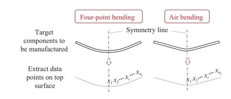
Fig.1. Examples of target components to be manufactured using four-point bending and air bending respectively and geometry representation for assessing the error between the designed and manufactured components. Only the data points of half of the geometry were used because of the symmetric shape.
2) Numerical Procedures
Fig.2 present the FE models and experimental setups for four-point bending and air bending. As can be seen in the FE model of the four-point bending in Fig.2(b), the punch is only allowed to translate along Y axis and given a displacement in Y direction. The Die is fixed, and the workpiece is symmetric about its symmetry line. The friction coefficients between tools and workpiece in both cases were set to be zero for simplicity.

Fig.2. The geometry, test setup and plane strain FE model for the fourpoint bending and air bending.
The specification of the experimental setup for four-point bending and air bending shown in Fig.2(a) is presented in Table I.
As these numerical experiments were performed in 2-D scale, plane strain element with quadratic geometric order was used to mesh the part of workpiece. In Abaqus 2019, it isdefined as CPE8R: An 8-node biquadratic plane strain quadrilateral, reduced integration. The components modelling the punch and die working face were meshed with undeformable mesh, while the workpiece was set to be homogeneous and modelled with deformable mesh. A total element number of 21 328 was used in the FE simulation, after a grid-independence study performed to determine the most appropriate mesh size which assures reasonable simulation accuracy with low computational time.
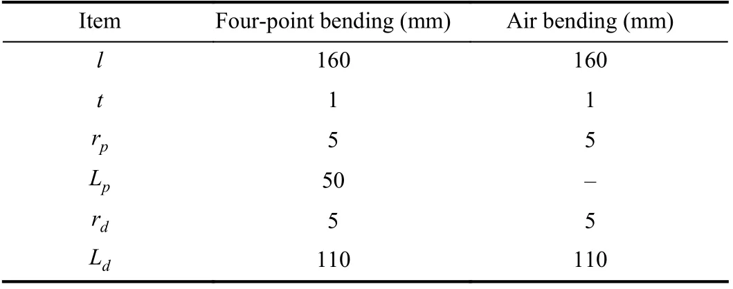
TABLE I EXPERIMENTAL SETUP DATA FOR FOUR-POINT BENDING AND AIR BENDING
3) Material Properties
The stress and strain curves of material of AA6082 and SS400 were extracted from [43], [44], with which the main properties of these materials were summarized and listed in Table II. The strain-hardening coefficient, n, and strength coefficient, K, were calculated by fitting the following equation to the data domain in log-scale stress-stain curve where plastic deformation occurs [45]

where σ is the true stress and ε is the true strain.
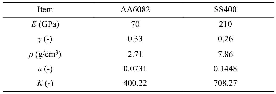
TABLE II VALUES OF THE PARAMETERS FOR THE MATERIALS INVESTIGATED
B. Network Training in the Intelligent Sheet Metal Forming System

Fig.3. The architecture of the ISMFS with the internal data flow.
Fig.3 shows the architecture of the ISMFS the DNNs were implanted, in which a database and a knowledge base were embedded. The database provides factual data to an FEA module where numerical computations are conducted to acquire the data for training of the TG-DNN. The learning of the DNN is guided by the prior knowledge or theories, which are stored in the knowledge base. After the DNN is trained to convergence, a new target workpiece geometry which is different from those in the training data is fed into the DNN through a user interface. A predicted stroke for the newly given geometry is then obtained from the DNN and used for another process simulation in the FEA module to yield the workpiece geometry after springback. Apart from obtaining the data from FEA simulations, experimental data could also be used as the training samples. In this research, all training data were obtained from FEA simulations. Finally, the data points representing the predicted and target workpiece geometry are compared to determine the maximum distance between them, which is denoted by ΔGEOMpred. The value of ΔGEOMpredmeasures the prediction accuracy of the whole learning system.
1) Training Data Design and Processing
The whole dataset for training and generalization evaluation was extracted from computational experiments, conducted in the FEA module shown in Fig.3, in which a total number of 201 simulations were performed with loading stroke ranging from 11 to 31 mm with an increment of 0.1 mm. The dataset is in a form of input-output pair, with input as the workpiece geometry representation data and output as the loading stroke.The output also includes physical parameters of true stress σ and true strain ε, which are acquired at the mid-point on the top surface of the workpiece before springback. Examples of the CAD of the desired workpiece after springback in fourpoint bending and air bending have been shown in Fig.1. The whole dataset was then randomly split into a training set and test set. Three different training to test data ratios were used in this research: 80%/20%, 50%/50% and 20%/80%. This composition of data was designed to evaluate the performance of the TG-DNN and the data-driven DNN with different amount of training data.
Modern DNNs, especially the convolutional neural networks (CNNs) in Computer Vision, have been proven to be able to localize and extract the important features from imagebased inputs, which have been confirmed to facilitate the learning of the relationship between input data and the outputs of interests [37], [46]. With the hindsight, the input in the whole dataset was designed to be in an image-based geometry representation, known as “grayscale map”, with a 1-D array containing the local depth value about the free-end of the workpiece. Within the “grayscale map”, grayscale-values(GS), ranging from 0 to 255, were used to encode the local depth. 0 GS (“black”) denotes the location at and beyond the free-end of the workpiece (no depth), while 255 GS (“white”)denotes the location with highest depth. To further improve the learning potential of DNNs, the input data were normalized by its highest value and the outputs were standardized in the output data domain.
Fig.4 presents some examples of inputs for the DNN in graphs and grayscale maps, respectively. It is noted that the transverse dimension in grayscale maps is used only for better visualization. There are in total 801 pixels in the longitudinal dimension, evenly distributed and aggregated to be the length of 80 mm (half length of the original workpiece blank). The map values were interpolated, with inverse distance weighting(IDW) interpolation method, from the computational results of coordinates along half of the top surface of the workpiece after springback, leveraging the symmetry of the workpiece shape.
2) Deep Neural Network

Fig.4. Examples of workpiece geometry representations (801 pixels).
A classic convolutional neural network was designed with the concept of multi-task learning as the DNN architecture,which is schematically shown in Fig.5. The inputs to the DNN are the greyscale maps extracted from the raw CAD data of the target workpiece after springback, and the outputs from the network include predictions of the required loading stroke and two physical parameters at the regularization spot before springback. TensorFlow Core v2.2.0 was used as the platform to establish and train the neural networks.
The convolutional layer utilizes the discrete convolution operation to shift the kernel function through the input space,which is defined as follow:


Fig.5. Architecture of the deep neural network in the ISMFS.

where θ*are the optimal θ to obtain the minimum value of the objective function at the end of the optimization. Several prevailing optimization algorithms have been developed to realize this calibration process over the last decades, with their different upsides and downsides. The commonly used learning algorithms include stochastic gradient descent (SGD) [33],Adam [48] and root mean square propagation (RMSProp)[49].
3) Parameter Norm Regularization
Regularization methods have been applied to traditional machine learning for decades, and they are proved to be also effective in limiting the capacity of DNNs after the advent of deep learning. Parameter norm regularization introduces a parameter norm penalty, αΩ(θ), to the original objective function shown in (7) and obtain a regularized objective function [33]

where α ∈[0,∞) is a hyperparameter used to control the relative contribution of the norm penalty term, Ω(θ),regarding to the original objective function, J(θ;X,Y). Θ represents all the parameters involved in this network,including weights, biases and hyperparameters. It can be seen that the penalty term is a function of trainable parameters, θ.By controlling the training modes of the network parameters,the overfitting issues in many research studies can be addressed or alleviated [33].
Theory-guided deep neural network respects prior treasurable theoretical or empirical knowledge by leveraging the theories to regularize the learning process. Compared to pure data-driven DNN model, a well-trained TG-DNN would be more than just a “black box” as theoretical knowledge is taken into account and the credibility of its prediction results is thus increased. Similar to the general form of the regularized objective function in (9), the theory-guided loss function is regularized by theoretical laws as shown as follow:

where αTH∈[0,∞) is a hyperparameter used to control the relative contribution of the theory-guided penalty term,JTH(θ;X), which is defined as


Swift’s law is a generalized power law for expressing the material-hardening behavior when plastic deformation occurs in a material [53], which has been introduced in (1). To replicate material model obtained in the one-dimensional tension test, a plasticity model is defined using a scalar equivalent stress and an equivalent plastic strain to replace the true stress and true stress in (1). The von Mises stress, σv, and the corresponding equivalent plastic strain, εeq, are used in this study

Thus, (12) is the theoretical equation used in this study to regularize the learning of the TG-DNN. Two extra tasks on learning additional physical parameters (true stress and true strain) are added to the TG-DNN for regularization.


Then the theory-guided objective function regularized by Swift’s law is given as follow:


The effectiveness of the introduced theory-guided penalty term, JTH(θ;X), is manually checked for the training examples by comparing the calculated values of the penalty term and the ideal value (zero). The calculation check was performed for the whole 201 data in the four experiments shown in Section III, with the relative error to the ideal value presented in Fig.6. It can be seen that the relative error for each training dataset is negligibly small, thus, the application of the theory-guided penalty to regularize the learning of the training data domain is theoretically valid.
4) Training Methods
For training the SVR, the radial basis function kernel was used, and the hyperparameters of “ ϵ” and “C ” were set as 0.1 and 1, respectively. The SVR was established and trained with scikit-learn library in Python. The Adam optimization algorithm [48] was used to train the DNNs, with default parameters of its hyperparameters (β1,β2,ϵ) in TensorFlow Core v2.2.0. The DNNs were trained with mini-batch training method [33]. At training, the training data were shuffled after each training epoch, which indicates one full cycle through the whole given training dataset, to reduce the sequence bias to the learning. The sizes of mini-batch used in different experiments are presented in Section III.

Fig.6. The relative error between the calculated results of the theoryguided penalty term for the whole 201 examples and the ideal value (zero) for the indicated materials and processes. 4-pt bend denotes four-point bending process.
An exponentially decaying learning rate was used in this research, as lower learning rate is recommended as the training progresses. The learning rate decaying scheme is defined as follow:

where η denotes the learning rate at the current decaying time step whose number is td, η0is the initial learning rate, sdis the decaying rate and Tdis the total decaying step number. sdand Tdwere set as 0.96 and 100 000 in this research.
The hyperparameters search space for the DNNs studied are presented in Table III. The highest test accuracy that the model can reach in these search domains would be regarded as the best performance the model can achieve.

TABLE III HYPERPARAMETERS SEARCH SPACE
C. Data Acquisition and Training Process
Fig.7 shows the training data acquisition through the FE simulation and how the data were used for TG-DNN training,which is taking place in the ISMFS as shown by the red dashed square in Fig.3. The experimental results of loading stroke ( ds) and two physical parameters ( σvand εeq) at the mid-point of the workpiece top surface were collected before the springback of the workpiece. Thus, only one regularization spot was set. These data were used as the target data in calculating the physics-guided objective function as shown in(14). The top surface geometry feature of the workpiece after springback was extracted and pre-processed to grayscale map before it was fed into the network as inputs.

Fig.7. Training data acquisition and data flow between FE simulation and TG-DNN training.
Fig.8 shows the iterations in the whole learning process to obtain the optimal loading stroke to manufacture the target workpiece. The difference between the geometry of the target workpiece and the workpiece manufacture with the predicted stroke, ΔGEOM, is evaluated in each iteration to update the parameters of the DNN. |ΔGEOM| is iteratively reduced through this learning process and would reach a minimum value in the end of the learning.
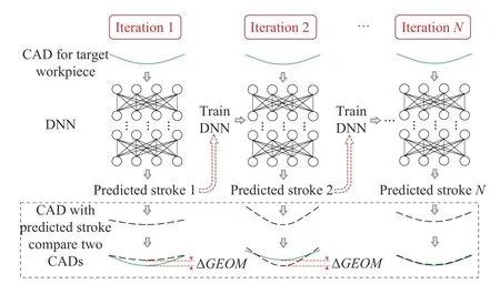
Fig.8. The learning process to obtain the optimal loading stroke prediction.
III. LEARNING RESULTS AND DISCUSSION
All the neural models were trained with the hyperparameters search space shown in Table III. The model that result in the lowest relative L2norm on the test set was then trained for another 3 times, and the generalization error of the network was obtained by averaging the performance of the three trained models. The average results of ΔGEOMpredfrom the three training is used to measure the performance of the machine learning models.
A. Comparison Between Support Vector Regression and Neural Networks
To evaluate the performance of the machine learning models described in the methodology section (SVR, datadriven DNN and TG-DNN), the original 201 data were split into three different training-test data composition: 80%/20%,50%/50% and 20%/80%. The training data were randomly sampled from the whole dataset for 10 times to train the models, of which the average results are shown in Fig.9. As the theory-guided learning exploits the concept of multi-task learning, to ascertain whether this method improves learning performance, two data-driven DNNs, multi-task DNN (MTDNN) and single-task DNN (ST-DNN), were established for comparison. The four DNNs used the same architecture as shown in Fig.5, except for the ST-DNN which only has one neuron in the output layer. All the machine learning models were applied to predict the loading stroke, based on the target workpiece geometry, in a four-point bending process of a sheet metal with material of AA6082. The number of trainable parameters for ST-DNN is 6 217 769, and that for MT-DNN and TG-DNN is 6 217 791.
From Fig.9, the prediction accuracy from SVR has apparent deterioration when the amount of training data is reduced,while those from the three neural models have negligible change. Furthermore, the predictions from DNNs conforms well with the true data in all three cases, while the prediction from SVR has clear deviation from its true data, especially when only 20% data were used for training. The results of the maximum distance between the target and predicted workpiece shape (ΔGEOMpred), which is used to measure the prediction accuracy, for the four machine learning models are shown in Table IV. From the results in the table, the datadriven models and the theory-guided model show indiscernibly good performance in all three experiments. To further evaluate the learning capability of the data-driven DNN and the TG-DNN, an experiment was performed with its results shown in the sequel.
B. Comparison Between Data-Driven DNN and Theory-Guided DNN
Because of the nearly equal performances of the data-driven and TG-DNN, another experiment was designed with new composition of training and test data. The ratio of training to test data is kept to the poorest condition as in last experiment(about 20%/80%), while the training data were chosen to eschew large continuous regions of data domain which were unseen at training, instead of having a relatively uniform data for training obtained from random sampling. Two data compositions, named symmetric (includes stroke values in the range of 11-12 mm, 21-22 mm and 30-31 mm) and asymmetric training data (includes stroke values in the range of 11-15 mm and 30-31 mm), were designed in this study. This design of training data is to better reflect practical situations in industry, where experimental data are expensive and scattered.In addition, to evaluate the learning consistency of neural models, two more experiments were designed to apply both data-driven DNNs and TG-DNN to 1) four-point bending process with a new material of SS400 and 2) air bending process with the same material of AA6082. Thus, the learning capabilities of the neural models were evaluated in experiments with three varying conditions:

Fig.9. Comparison between the true data and predictions of the data domain from SVR, ST-DNN, MT-DNN, and TG-DNN, which were trained with data of three different ratios of training to test data. The true data were obtained from four-point bending test of AA6082. The training data were randomly sampled from the whole dataset.

TABLE IV COMPARISON OF THE AVERAGE OF THE MAXIMUM DISTANCE BETWEEN THE TARGET AND PREDICTED WORKPIECE SHAPE(ΔGEOMPRED) FROM THE WELL-TRAINED SVR AND DNNS EVALUATED ON THE TOTAL DATA DOMAIN (MM)
1) Different raw data structure: using symmetric/asymmetric training data, which were acquired from the four-point bending process of the AA6082 workpiece.
2) Different workpiece material: using symmetric training data, which were acquired from the four-point bending process of the SS400 workpiece.
3) Different forming process (applications): Using symmetric training data, which were acquired from the air bending process of the AA6082 workpiece.
Fig.10 shows the training loss curves for the three DNNs during training and their generalization performance under four different conditions. The generalization performance is measured by evaluating the well-trained DNN on the test set,and the predictions for the whole data domain from different models are plotted. It was seen that the training losses of DNNs in different cases all converge to a small value at the end of training. Due to an extra theory-guided regularization term in the objective function for the TG-DNN, the convergence of which would conflict that of the standard objective function, the converged training loss of the TGDNN are larger than those of the pure data-driven DNNs.From the prediction curves of the three models, compared to the performance of the DNNs trained with randomly sampled training data in Fig.9(a), the prediction from the TG-DNN remains a good fitting to its target value, while the data-driven DNNs trained with scattered data in this section fail to learn the true function in the unsupervised data domain in most experiments. Besides, the TG-DNN shows a good learning consistency from its consistent performance under various training conditions and in different applications. Table V shows the average results of ΔGEOMpredfrom the DNNs in all experiments, in which the TG-DNN is superior to the two data-driven DNNs. It is worth noting that the MT-DNN outperforms the ST-DNN in most cases, which indicates that the learning of loading stroke could be improved by learning extra tasks of local true stress and strain.
C. Learning With Scarce Training Data
In industry, experimental data can be rather expensive, for which of great significance is the predictive model to have a good performance with very limited training data. Thus, in this section, a new experiment was designed to have a total number of 21 examples of dataset, with loading stroke ranging from 11 to 31 mm with unit increment. The whole dataset was then split into a training set and test set, with data pairs with odd numbers of loading stroke (i.e., 11, 13, 15, 17, 19, 21, 23,25, 27, 29, 31 mm) as training set and data pairs with even numbers of loading stroke (i.e., 12, 14, 16, 18, 20, 22, 24, 26,28, 30 mm) as test set. Thus, there are in total 11 and 10 data examples in training set and test set, respectively. To comprehensively evaluate the performance of the DNNs with scarce data, three different amounts of training data were used for training the neural networks. The original training set with 11 examples were designed to be the “full training set”.Likewise, the training data with 6 (with stroke values of 11, 15,19, 23, 27, 31 mm) and 3 (with stroke values of 11, 21, 31 mm)evenly distributed examples are referred to as the “half training set” and “1/4 training set”.
All the networks were trained to convergence with the batch size of 2. Fig.11 presents the generalization results of the STDNN, MT-DNN and the TG-DNN, well-trained with full and half original training data, on the test set. The training data were obtained from the four-point bending process of AA6082 workpiece. It can be seen that, with full and half amount of training data, all DNNs perform nearly equally well. This can also be observed in Table VI, in which the values of ΔGEOMpredbetween the target and predicted workpiece geometry from all models are negligibly small with full and half training data.

Fig.10. The training loss curves for the three DNNs (upper row) and the evaluations of the DNNs on the total data domain (lower row) after training with about 20% training data acquired from different applications. The training data was designed to be symmetric and asymmetric to have large continuous regions of missing data domain.

TABLE V COMPARISON OF THE AVERAGE OF THE MAXIMUM DISTANCE BETWEEN THE TARGET AND PREDICTED WORKPIECE SHAPE (ΔGEOMPRED)FROM THE WELL-TRAINED DNNS EVALUATED ON THE TOTAL DATA DOMAIN IN ALL EXPERIMENTS (MM)
With 1/4 training samples, the training data were also designed to be structurally symmetric (includes stroke values of 11, 21 and 31 mm) and asymmetric (includes stroke values of 11, 13 and 31 mm) for four-point bending of AA6082 like in Section III-B. The models were also applied to applications of 1) four-point bending process with a new material of SS400 and 2) air bending process with the same material of AA6082 to comprehensively evaluate the performance and learning consistency of the data-driven DNNs and TG-DNN.

Fig.11. Comparison of generalization capability on test set between the data-driven and theory-guided DNNs with (a) full data; (b) half data, obtained from four-point bending process of AA6082 workpiece.

TABLE VI COMPARISON OF THE AVERAGE OF THE MAXIMUM DISTANCE BETWEEN THE TARGET AND PREDICTED WORKPIECE SHAPE (ΔGEOMPRED)FROM THE WELL-TRAINED DATA-DRIVEN AND THEORY-GUIDED DNNS EVALUATED ON THE TEST SET.THE DATA WERE OBTAINED FROM FOUR-POINT BENDING PROCESS OF AA6082 WORKPIECE (MM)
Fig.12 shows training loss curves for all the DNNs during training and the generalization performance of them under four different conditions. The generalization performance is measured by evaluating the well-trained DNN on the test set(with stroke values of 12, 14, 16, 18, 20, 22, 24, 26, 28, 30 mm).It was seen that the training losses of all the DNNs in different cases all converge to a small value at the end of training.Similar to the results in experiments with 201 total data shown in Fig.10, the TG-DNN has a higher converged loss than the data-driven DNNs due to its extra theory-guided regularization term in the objective function. From the prediction graphs, the predictions of stroke values on the test set from the TG-DNN have a good match to the target values in all cases. Compared with the multi-task and single-task learning results, where generalization errors occur evidently,the TG-DNN exhibits effective learning and still holds high generalization performance in the data domain away from the training set. With only 1/4 training data, the data-driven DNN fails to learn the true function in the unsupervised data domain, while the TG-DNN succeeds to retain high learning capability. From the average results of ΔGEOMpredin different applications shown in Table VII, with 1/4 training data, the results of ΔGEOMpredmeasured from TG-DNN only have an increase less than 0.1 mm than those obtained from training with full and half data shown in Table VI. Thus, the TG-DNN exhibits a significantly more robust and consistent learning capability than data-driven DNNs when applied to problems with different data structures and amount of the training data,different materials of the workpiece and different bending processes.
It is worth noting that, in the case with asymmetric training data shown in Fig.12(b), the TG-DNN also managed to learn the true function in spite of the considerably increased learning difficulties due to large amount of missing data domain for training purpose (between target stroke of 13 and 31 mm). The predictions from both MT-DNN and ST-DNN have evident deviation from the true function in this region. It is well known that the structure of the training dataset has significant influence on the training of neural networks, while the data structure is commonly irregular when acquiring offthe-shelf experimental data. Thus, the introduced TG-DNN, in practice, can effectively alleviate the demand on the amount and structure of expensive experimental data, which could reduce the effort in experiment design. Also, from the prediction graphs in Figs. 10 and 12, the performance of the data-driven DNNs trained with only three examples in Fig.12 is inferior to that of the DNNs trained with 30-50 data in Fig.10, while the TG-DNN shows a more consistent performance. This indicates the superior learning capability of the TG-DNN than the data-driven DNN trained with very scarce data. It should be noted that other efforts have also been made to deal with missing data values, such as nonnegative latent factor model [54], [55], which outperforms the state-of-the-art predictors.
Taking case 1 and case 4 (Figs. 12(a) and 12(d)) as examples, with the predicted values for target stroke of 24 mm from the DNNs, the obtained workpiece geometries deformed by four-point bending and air bending are compared with their targets, as shown in Fig.13. It can be seen that the geometry predicted from TG-DNN is evidently closer to the target than those from ST-DNN and MT-DNN. Fig.13 also shows how the ΔGEOMpredis measured for different DNNs.
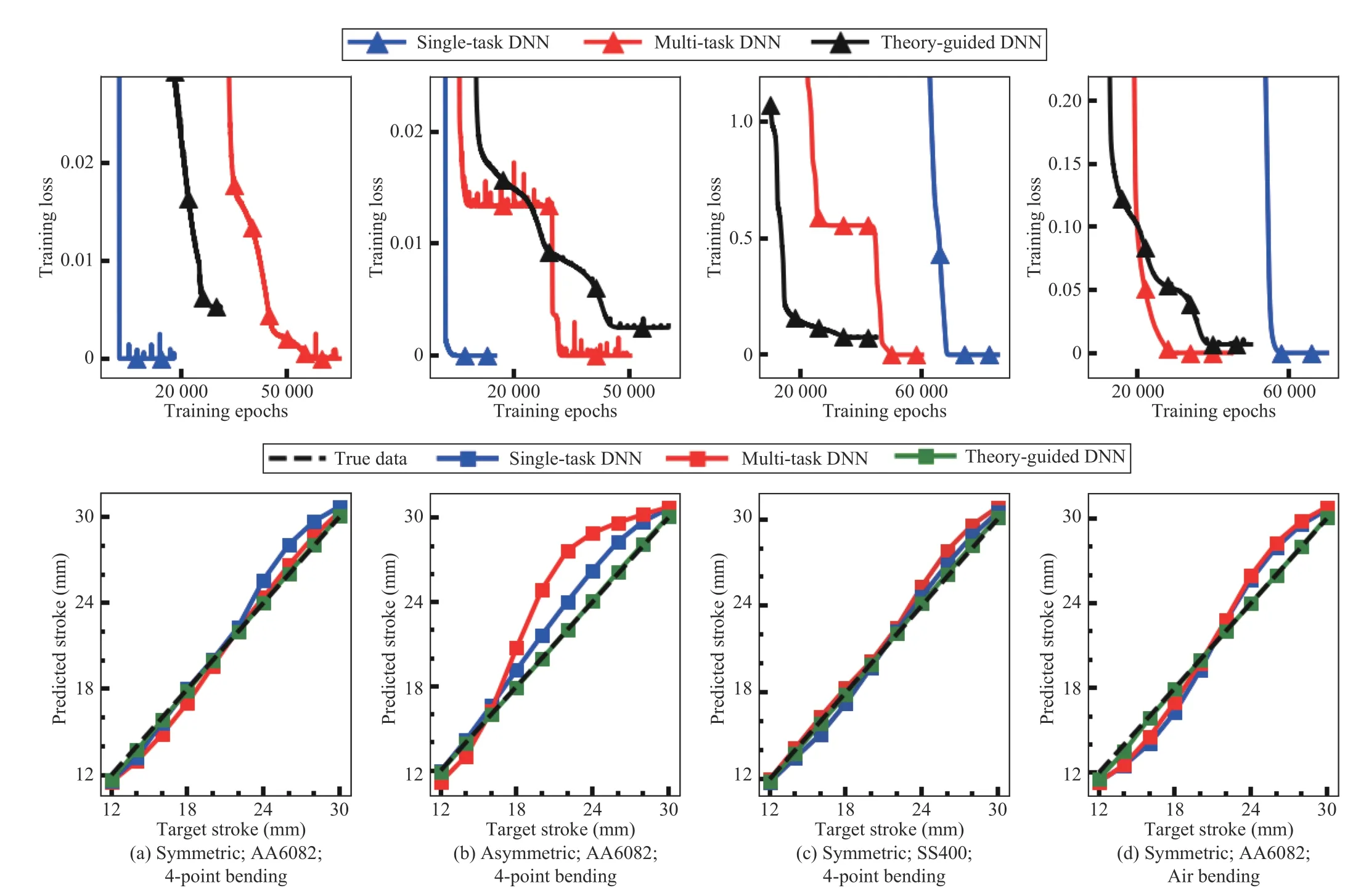
Fig.12. The training loss curves for the data-driven and theory-guided DNNs (upper row) and the evaluations of all the DNNs on the test set (lower row)after training with 1/4 training data acquired from different applications.

TABLE VII COMPARISON OF THE AVERAGE OF THE MAXIMUM DISTANCE BETWEEN THE TARGET AND PREDICTED WORKPIECE SHAPE (ΔGEOMPRED)FROM THE WELL-TRAINED DATA-DRIVEN DNNS AND THEORY-GUIDED DNN EVALUATED ON THE TEST SET IN ALL EXPERIMENTS (MM)
To ascertain whether the generalization accuracy of the DNN is promoted by the proposed theory-guided regularization method using Swift’s law, the final training loss and test loss of the physical parameters ( σvand εeq) from the well-trained TG-DNN and the MT-DNN in all experiments are compared as shown in Fig.14. It can be seen that the training loss of these parameters from data-driven DNN are extremely smaller than those from the TG-DNN, which is due to the convergence conflict between the standard term and the theory-guided term in the objective function for the TG-DNN.However, the loss of the physical parameters on the test set from the TG-DNN are smaller than those from the data-driven DNN, which indicates its better learning outcome in the physical-parameters data domain. This corroborates the learning improvements introduced by the TG-DNN, as the physical parameters were directly regularized in the theoryguided objective function. Consequently, the superior performance of the TG-DNN than the data-driven DNN is demonstrated by the introduced theory-respecting regularization method. With the effective implementation of Swift’s law for training regularization, the interpretability of the DNN is improved.
In summary, the ISMFS with the novel TG-DNN proposed in this research has shown many advantages. The successful application of TG-DNN to sheet metal bending processes also indicates its applicability to other sheet metal forming techniques, where the physical parameters ( σvand εeq) are, in general, monotonically related to the forming parameters.Despite of its versatility, TG-DNN could also have limitation.As the learning task of interest is not directly related to the inputs to the model with a hard theory-respecting regularization function like those in [38]-[41] due to the inherent complexity of sheet metal bending engineering problems, a more tricky process of hyperparameters tuning than those for PINN could potentially be needed. As a consequence, the method would increase the computational cost compared to the PINN with PDE governing equations.However, because of the infeasible application of PINN in this research, discussion on these two neural networks could be futile.
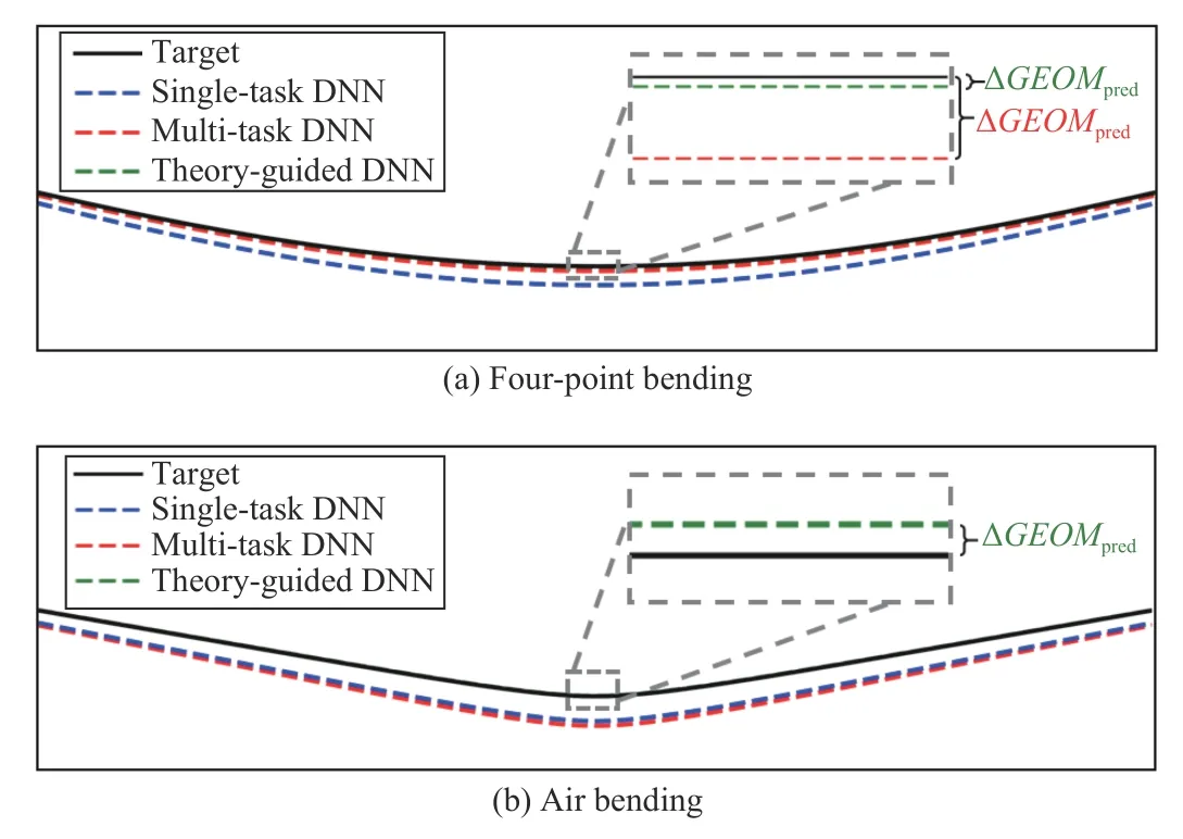
Fig.13. Comparison between the shape of the target workpiece (with target stroke of 24 mm) and the workpiece manufactured with the stroke predicted by the data-driven and theory-guided DNNs, which were trained with 1/4 symmetric data acquired from mid-point of the AA6082 workpiece from(a) four-point bending and (b) air bending.
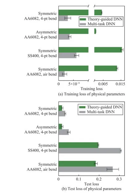
Fig.14. Comparison between the training and test loss of physical parameters ( σv and εeq) between well-trained MT-DNN and TG-DNN with 1/4 symmetric training data acquired from mid-point of the AA6082 workpiece from 4-point bending.
IV. CONCLUSIONS
In this research, a novel theory-guided regularization method for DNN training, embedded in a learning system, has been proposed. The TG-DNN, which utilizes Swift’s law as the guidance, improves the learning performance by regularizing the learning of extra tasks. A series of studies have been performed to evaluate the machine learning models,including a support vector regression model, two data-driven DNNs and a TG-DNN, in learning the intrinsic relationship between the deformed workpiece geometry after springback and the corresponding forming parameter of loading stroke.The following conclusions can be drawn:
1) The neural networks, either trained in data-driven or theory-guided, exhibit blatantly better learning capabilities than a traditional machine learning model, SVR, in predicting the loading stroke of a four-point bending and an air bending process. With less training data sampled randomly, the performance of the SVR deteriorates sharply, while those of the neural models have negligible decrease.
2) The proposed TG-DNN outperforms the conventional pure data-driven DNN for its superior generalization accuracy,when only scarce and scattered experimental data are available for training. When decreasing the amount of training data to a very small value (from 30-50 to 3 in this research),the performance of the data-driven DNNs suffers while that of the TG-DNN retains consistent.
3) With varying experimental conditions, including the structure and amount of training data, workpiece material and sheet metal forming application, the TG-DNN exhibits a more robust learning capability and learning consistency than the data-driven DNNs.
4) Other than bending, The TG-DNN could also be applicable to the sheet metal forming processes where the physical parameters ( σvand εeq) are, in general, monotonically related to the forming parameters. The theory-guided learning also improves the interpretability of the traditional data-driven DNNs.
5) Consequently, in practice, the proposed theory-guided regularization method could potentially relieve the high demand on the amount and structure of expensive experimental data. Furthermore, by implementing the theoryguided deep learning technology, the problems of considering springback in the traditional design of sheet metal bending processes could be circumvented. The TG-DNN, thus,provides an alternative method for compensating springback with significantly shorter development cycle and less capital cost and computational requirement than traditional compensation methods which are based on FE simulations and experiments.
One of the future works is to apply this TG-DNN to other sheet metal forming processes. Developing a harder regularization method, by introducing new or more theories for sheet metal bending process and/or increasing the regularization spots in the theory-guided objective function,could also be worthy of investigation. Also, the latent relationship between the process parameters and the workpiece geometry after springback could be learned by developing equations, which could be transformed from equations describing the workpiece-tools topology before springback by adding a to-be-learned term relating the workpiece geometry before and after springback. Other approaches could be used to enhance the theory-guided model, with more advanced optimization methods [56], [57],or discrete-time delayed neural networks [58], [59].
杂志排行
IEEE/CAA Journal of Automatica Sinica的其它文章
- Ground-0 Axioms vs. First Principles and Second Law: From the Geometry of Light and Logic of Photon to Mind-Light-Matter Unity-AI&QI
- Nonsingular Terminal Sliding Mode Control With Ultra-Local Model and Single Input Interval Type-2 Fuzzy Logic Control for Pitch Control of Wind Turbines
- Deep Learning for EMG-based Human-Machine Interaction: A Review
- Distributed Secondary Control of AC Microgrids With External Disturbances and Directed Communication Topologies: A Full-Order Sliding-Mode Approach
- Autonomous Control Strategy of a Swarm System Under Attack Based on Projected View and Light Transmittance
- Computing Paradigms in Emerging Vehicular Environments: A Review
