ST-Trader: A Spatial-Temporal Deep Neural Network for Modeling Stock Market Movement

Xiurui Hou, Kai Wang, Cheng Zhong, and Zhi Wei, Senior Member, IEEE

Abstract—Stocks that are fundamentally connected with each other tend to move together. Considering such common trends is believed to benefit stock movement forecasting tasks. However,such signals are not trivial to model because the connections among stocks are not physically presented and need to be estimated from volatile data. Motivated by this observation, we propose a framework that incorporates the inter-connection of firms to forecast stock prices. To effectively utilize a large set of fundamental features, we further design a novel pipeline. First,we use variational autoencoder (VAE) to reduce the dimension of stock fundamental information and then cluster stocks into a graph structure (fundamentally clustering). Second, a hybrid model of graph convolutional network and long-short term memory network (GCN-LSTM) with an adjacency graph matrix(learnt from VAE) is proposed for graph-structured stock market forecasting. Experiments on minute-level U.S. stock market data demonstrate that our model effectively captures both spatial and temporal signals and achieves superior improvement over baseline methods. The proposed model is promising for other applications in which there is a possible but hidden spatial dependency to improve time-series prediction.

I. INTRODUCTION

THERE is strong evidence that stock prices of firms that interact with each other move together due to several reasons. First, exchange-traded funds (ETFs), such as S&P 500 and NASDAQ, track the prices of a basket of stocks.When people trade those funds, all the underlying stocks are traded simultaneously, which causes common fluctuations of those stock prices [1]. Second, most professional portfolio managers are specialized in a couple of strategies and these strategies often involve a similar set of stocks. For example,value investing [2] tilts to firms with high earning-to-price ratio, while momentum strategy focuses on firms with higher returns during the past year. On the one hand, any fundamental shock can affect the prices of a group of stocks together. The ongoing COVID-19 pandemic struck the traveling industry harder than the technology sector, so we observed stocks within the traveling industry fall significantly and simultaneously while those of tech companies did not drop much. On the other hand, portfolio managers may adjust their positions due to idiosyncratic reasons, for example, the price target predicted by their own model changes. Third,some companies have cooperative relationships, like Apple and Nvidia. If one of them has good or bad news, the effect on the other one could be reflected in the stock price. To our best knowledge, however, we have not seen an algorithm effectively incorporating these hidden dependencies among firms into the stock price forecasting task.

Although the interaction among companies is not difficult to observe, it is not easy to have it cooperated in stock prices forecasting tasks due to three reasons: 1) there are too many fundamental variables to select from (usually the total is more than 1000). Extra financial expertise is needed to filter out the key variables; 2) although the key variables are selected, the interaction imposed by those variables is not trivial to model due to nonlinearity and chaos; 3) the way that interaction contributes to the final forecasting goal is the biggest obstacle to utilize the fundamental information because such static information has different frequencies and scales from timevarying price variable.

Deep learning is well deployed in grid and sequence structured data, like image recognition in autonomous driving[3] and natural language processing [4]. However, graphformed data is more common but more complex in the realworld, like social relationships, sensor networks in smart cities, and stock connections in the financial market. Recently,there has been a surge of attention on graph representation, for example, link prediction, graph classification, and node classification. Motivated by the graph representation employed by previous studies, we propose a framework that models the hidden dependency among firms as a graph.

In the field of graph representation learning, tasks with onhand graph information are well-studied. For example, [5]used convolutional neural networks (GCNs) to improve recommendation systems; [6] used GCNs to learn material properties from the connection of atoms directly to predict density. However, those frameworks cannot be directly applied to the stock price forecasting since it is mainly a timeseries problem. Even though the stocks can be seen as nodes in a graph, edges among nodes are not trivial to define because there is no spatial locality attribute for each stock.Besides, forecasting stock price is a challenging task due to its tumultuous nature, which prevents the transfer learning from time-series tasks with apparent seasonality or trend. Due to such irregularities, the direct application of existing graphrelated models to the stock market is not appropriate.

In this work, we propose a hybrid deep learning pipeline,VAE-GCN-LSTM, to incorporate the graph structured relationship among firms into time-series forecasting tasks.The main contributions of this paper can be summarized as follows:

1) We design a variational autoencoder (VAE) to learn the lower-dimension latent features of companies’ fundamental variables to calculate more meaningful distance among companies, which helps construct the graph network.

2) We develop a hybrid deep neural network of graph convolutional network and long-short term memory network(GCN-LSTM) to model both the graph structured interaction among stocks and the stock price fluctuations on the timeline.

3) To evaluate the contribution, and the improvement of additional features, and the proposed method, we conduct comprehensive experiments on both predicting numerical stock price and binary stock price movement on a real dataset.

We consider the largest 87 firms listed in the United States in our experiment. These firms are included in the S&P 100 index and we only incorporate 87 out of 100 firms due to the data availability. Fig. 1 shows the underlying connections among these firms. In Section III we introduce how we take the connections among firms into account in the price forecasting task, and the actual performance is presented in Section IV.

II. RELATED WORK

A. Classic Approaches in Stock Market

Many factors and firm characteristics are demonstrated to be effective in forecasting stock prices [7]. For example,financial practitioners and fund managers have been following value investing strategies after, or even prior to, the publication of “The Intelligent Investor” [8] in 1965. Since then, exploring effective factors became a hot topic and a slew of factors have been explored. Examples of these factors include the book-to-market value of a firm [9], price-toearnings ratio [10], relative strength trading strategies that focus on the recent stock return of a firm [11], and the profitability and investment of a firm [12]. These factors possess valuable predictive power in terms of forecasting a firm’s future return.

The advent of advanced machine learning methods makes the stock return forecasting problem a more competitive task.Time-series and cross-section regressions are no longer the only toolkit we are able to utilize. For instance, [13] applied support vector machine (SVM) on forecasting NIKKEI 255 index’s movement on a weekly basis. In another independent work, [14] predicted the stock price movement of Taiwan(China) companies. Reference [15] used Random Forest to forecast the future stock prices and find it outperforms both artificial neural networks (ANNs) and SVM.

B. Deep Learning Approaches in Stock Market

Deep learning has achieved exciting performance in many areas, e.g., image recognition task [16] and natural language processing task [17]. The application of deep learning also includes stock price forecasting. Both the absolute price or return (numerical prediction) and the price movement (binary classification) are popular forecasting goals for researchers.Fully connected neural networks are applied to predict future stock price in Chinese market [18] and Canadian markets [19],and to predict stock return of Japan Index [20] and S&P500[21]. Long-short term memory (LSTM), which is designed to work on time-series tasks, is used in this forecasting problem[22], [23] since the stock price can be seen as a time series sequence. In the comparison results, LSTM has been demonstrated to outperform the fully connected neural networks.

Hybrid models, which take various sources of information to enrich the predictive power of the conventional machine learning algorithms, make the forecasting task more promising in recent years. For example, [24], [25] proposed a combination of wavelet technique and neural networks.Reference [26] introduced a hybrid model that combines autoregressive moving average models and artificial neural networks. A more recent work by [27] ensembled machine learning methods and financial technical analysis. In some related fields, like crowdfunding [28] and user intended action prediction [29], the hybridization of different types of neural networks has been applied successfully potentially due to its ability in accommodating heterogeneous input features.Reference [30] proposed a hybrid model combining long-short term memory and deep neural network (LSTM-DNN) for a stock forecasting task. This hybrid model, LSTM-DNN, first integrates static firm fundamental features into a time-series forecasting task. Refer to [31]–[34] for more hybrid models on forecasting problem. However, no matter how the neural network structure changes in the literature above, none of them takes the interactions among firms into consideration in the prediction task. It is intriguing to extract these implicit interactions and use them as input for the forecasting tasks.

C. Convolutional Neural Networks in Graph-Structure Data

Recently, applying convolutional neural networks (CNNs)to graphs with arbitrary structures has caught people’s attention. Two main directions are being explored in the literature: 1) the definition of spatial convolution is generalized in [35], [36]; 2) generalizing CNNs to 3-dimensional data as a multiplication in graph Fourier domain is discussed in [35], [37], [38] by the way of convolution theorem. Using geodesic polar coordinates, the authors define the convolution operation on meshes. Therefore, this method is suitable for manifolds and cannot be directly applied to graphs with arbitrary structures. The spatial approach proposed in [36] has more potential possibilities in generalizing CNNs to arbitrary graphs. It has three steps: first,select a target node; second, construct the neighborhood of target node; third, normalize the selected sub-graph by ordering the neighbors. The normalized sub-graphs are then fed into 1-dimension Euclidean CNN. Since there is not a natural ordering property in graphs, either temporal or spatial,it has to be imposed by a labeling procedure. The spectral framework to solve this issue is first introduced by [37] and is described in Section III-D. The main disadvantage of this method is the high computational complexity, O(n2). To overcome this problem, [38] provides strictly localized filters with a linear complexity O(|E|). The first order approximation of the proposed spectral filter is adopted by [39] in a semisupervised node classification task. Thus, we also use the spectral filters introduced in [38] in our framework because of the efficiency and denote the convolution operation as ∗G.

Applying graph convolution operation in time-series tasks is demonstrated to be helpful in some studies. Reference [40]developed a spatio-temporal GCN model for traffic forecasting. The conventional method for traffic forecasting is to do time-series analysis for each traffic entity, like a specific highway or a city road. The more natural thought is that if two roads are close, they have high probability to experience the same volume of traffic. In their study, the GCN model can perform convolution operation with much faster training speed and fewer parameters than the traditional CNN model that is more suitable for grid structured data, e.g., images.Reference [41] also proposed a spatio-temporal GCN model for human body skeletons based action recognition and the improvement is significant. Reference [42] used GCN in dynamic texture recognition by extracting low-level features.Reference [43] combined LSTM and convolutional LSTM for capturing both time sequencing features and map sequencing features. There are some attempts to combine time-series forecasting and graph structured convolution operation, like[44] and [45] forecasting wind speed and solar radiation by enriching the time-series with wind farm distances and solar site distances. The wind farms located nearby are supposed to experience much the same wind speed and direction. Wind forecasting tasks benefit from the geographical information via graph convolutional network.

III. METHOD

In this section, westart with the pr oblem formulation of prediction task with spatial and temporal dependencies. Then,we use VAE to reduce dimensions of fundamental feature space and generate the spatial graph structure for the selected stocks. After that, we introduce a spatial-temporal model,GCN-LSTM, to predict the future stock prices.

A. Problem Formulation

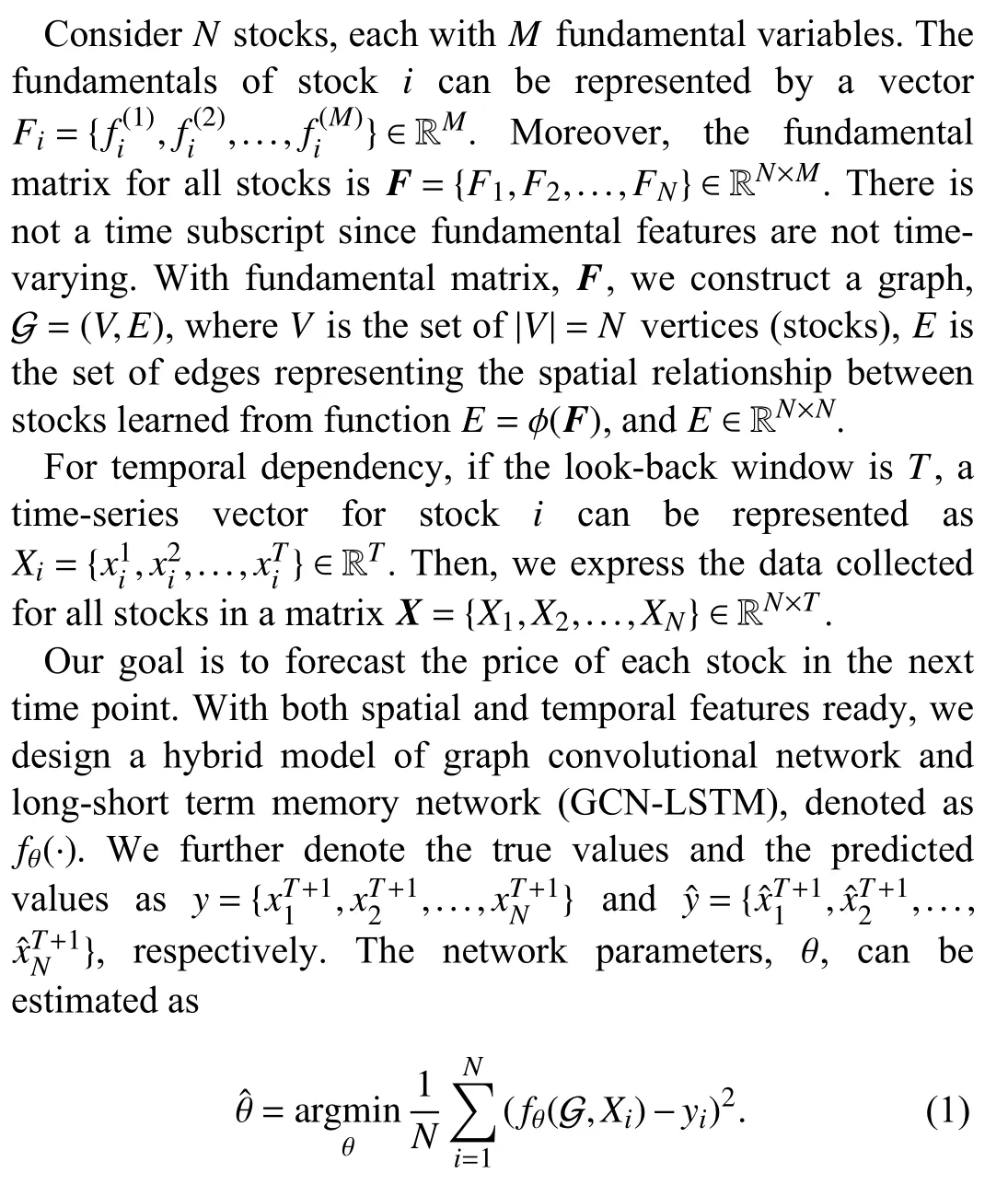
B. Variational Autoencoder

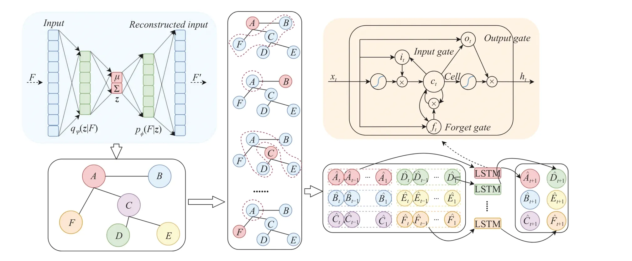
Fig. 2. Spatial-temporal modeling using GCN-LSTM framework for unspecified spatial graph structure. The area shaded in green is the VAE that reduces the dimension of the fundamental feature to learn more meaningful distance among stocks. The network below it is the constructed graph based on the learnt distance. The vertical panel to the right of VAE presents the convolution neighbors of each node. The area shaded in yellow is the network of a LSTM cell. The time-series inputs enriched with fundamental signals by convolution operation are fed into a LSTM network for final predictions.

C. Long-Short Term Memory (LSTM)

In Fig. 2, the construction of LSTM is represented in the area shaded in yellow color which is located in the upper-right corner. A compact form of the equations for the forward pass of a LSTM unit with a forget gate is represented below:

D. Graph Convolutional Networks

E. ST-Trader: Spatial-Temporal Modeling Using GCN-LSTM Framework

We propose to incorporate the spatial signal into time-series prediction with graph convolutional network. The global spatial dependency learnt via VAE is represented by the adjacent matrix, A, calculated from the features from lowdimensional latent space. For notational simplicity, let∗Gxtdenotes a convolution operation on xtwith filters (kernel size:dh×T ) that are functions of the graph Laplacian L, as noted in(14). By replacing the original inputs with convolutionapplied inputs, the equations of GCN-LSTM cell are given as follows:

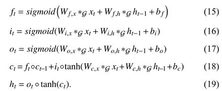
In our setting, W.,h∈RK×dh×dhare the Chebyshev coefficients that defines the support of the graph convolutional kernels.W.,h∈RK×dh×dhdetermines the number of parameters that is independent to the number of nodes in the graph. Parameter determines the number of neighbors used to compute the aggregated states for any target node so that it also determines the communication overhead in a distributed computing setting. The detailed algorithm description is shown in Algorithm 1.

Algorithm 1 Training Process for the ST-Trader F ∈RN×M M N Input: . Fundamental feature matrix with variables for stocks;X ∈RN×T T N. Time-series feature matrix with look-back window for stocks;γ2=0.1ϵ=0.5 256 K=3 E=1000 h=16 d=3; ; minibatch size ; polynomial order ; number of epochs ; the hidden space dimension ; network depth .ϕ ψ θ Parameters: , of VAE; of GCN-LSTM.ϕ , ψ ← Initialize parameters;repeat g ←∇ϕ,ψL(ϕ,ψ;F)(Gradients of minibatch estimator of (3));ϕ,ψ ← g 1e−5 Update parameters using gradients with learning rate =and Adam optimizer [48];until convergence of parameters ( );A ϕ,ψ The adjacent matrix for the edge information in Distance of latent features derived by the VAE using parameters ;G ←ϕ,ψ

˜L ←Calculate rescaled Laplacian using A;θ ←Initialize Initialize parameters;e ←1;e ≥E while do X′← ∗G apply convolution operator on X using (14);ˆy ←LS T M(X′);Update , , and in by gradient descent using (1) with learning rate = and RMSprop optimizer [49];e ←e+1 Wx.Wh. b θ 1e−5

IV. ExPERIMENT

A. Data Description

Since we consider the spatial dependency among firms, the number of our training samples is divided by the number of firms. For example, suppose we have 10 firms and 100 observations for each firm. The total number of samples is 1000 if we take firms independently but the number drops to 100 if we consider the relations among firms. To obtaining enough samples, we use minute-level stock data of 87 firms from S&P 100 composite in 2010 due to the availability of data. The number of total minute-observations is 97 890, and we split the whole dataset into batches using the sliding window. We also check the robustness of our results using five-minute-interval stock prices, which guarantees enough samples for at least one epoch training and testing. For fiveminute-interval, the sample sizes of training, validation, and testing set are 16384, 2944, 2944, respectively. The used fundamental variables and stock tickers are presented in Appendix. For categorical variables such as SEC and SIC, we use their one-hot encoding as input for VAE to learn the latent feature.

B. Experimental Settings

For one-minute-level data, the testing period is one month after the training period. For example, if the testing is Feb 2010, the training data would be Jan 2010. The last testing period is Dec 2010. Thus, we have 11 testing periods and the number of samples for each month is listed in Table I.

Algorithms studying on daily data may cover a period of many years, since one year has around 250 trading dates (data points) only. However, as shown in Table I one month can have more than 7000 minute-level samples/data points. We note that the months in 2010 cover different market scenarios,such as uptrend (e.g., March), downtrend (e.g., August), and mixed (e.g., June) ones. Therefore, the minute-level data of year 2010 are representative of different market scenarios and sufficient for model validation.

To demonstrate the benefit of incorporating the spatial dependency among stocks on price forecasting, we consider the following baseline methods: 1) LR: For the classical linear regression model, we treat the historical time series prices as explanatory variables and the price of the next time point as the response variable; 2) FCNN: The fully-connected neural network which captures the non-linear relationship between time-series features; 3) LSTM: Long-short term memory neural network which contributes partially to the proposed method; 4) ecldn_ST-Trader: “ecldn” means calculating theEuclidean distance between a pair of stocks using the original fundamental variables. The spatial relationship in this setting is expected to be much noisier than using VAE; 5) idsty_STTrader: “idsty” means “industry”. The adjacent matrix for this method is derived from the industry category.Aij=1 means company i and company j are in the same industry category. The proposed model is denoted as vae_ST-Trader when compared to those baselines methods because it differs in deriving the adjacent matrix via VAE. The purpose of studying baseline methods 4) and 5) is to evaluate the ability of VAE to extract latent features from high dimension feature space. The network structure and the hyperparameters for all methods, are tuned using the validation set and the final performance results are derived on the testing set.

TABLE I NUMBER OF SAMPLES FOR EACH MONTH

We apply all methods mentioned above to forecast two targets: the numerical stock price and the binary price movement indicator (the label is 1 if price goes up from last time point and 0 if price goes down from last time point).Since deep neural networks are not stable when predicting unbounded numerical results, we scale both the training set and testing set using MIN-MAX normalization (see (20)) by the maximum and minimum value of the training set.

C. Evaluation Metrics

For the numerical stock price prediction, we adopt widely used metrics for real-valued prediction problems [50]–[53].They are defined as follows:

1) Mean absolute value percentage error (MAPE):

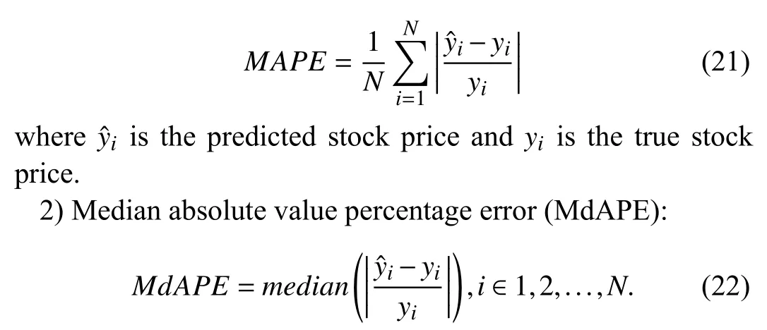
MdAPE sits around the median value of the data and is thus more robust to outliers compared to MAPE.

For the binary price movement prediction, we use area under roc curve (AUC) and other following metrics, (TP for true positive, TN for true negative, FP for false positive, and FN for false negative):

D. Results

1) Predicting Stock Price: Table II presents the MAPE and MdAPE for all testing periods. The stock price has been demonstrated to have extensive outliers because MdAPE is usually less than MAPE. The methods enriched with spatial information achieve better prediction results than temporalonly models. The proposed model, vae_ST-Trader,outperforms baselines across the board. Moreover, LSTM is more desirable than LR and FCNN in most batches.Interestingly, idsty_ST-Trader with only industry information is more preferable than ecldn_ST-Trader, which incorporates much more fundamental information. One possibility is that simple Euclidean distance calculated from all fundamental variables brings more noise to the spatial signal because it assigns equal weight to each variable. The contribution of each variable to the final prediction is hard to be quantified by the linear model. Clearly, extracting the latent interaction(spatial distance on the latent features) among firms using VAE benefits the prediction accuracy substantially.

2) Prediction Stock Price Movement: Fig. 3 presents the Accuracy and AUC scores of different methods on binary movement prediction chronologically. The Efficient-market hypothesis1https://en.wikipedia.org/wiki/Efficient-market_hypothesisstates that asset prices reflect all available information, and so there is not much space for algorithms to forecast stock prices. This hypothesis is supported by the poor accuracy in our study (Fig. 3) and in other literature. Although many investors apply value-investing strategies, which tie the market price of a stock to its underlying fundamental value,many other investors keep adopting technical analysis; they make trading decisions based on reading charts of the historical price trends. Therefore, there is still room for the methods to improve their predictive power if they do not take the influence of the technical-analysis trader on stock price into account. The proposed model is enriched by the extracted relationship among the firms so that it can better capture the trend signal compared to baseline methods. This advantage is reflected by both Accuracy and AUC scores.

The flash crash on May 6, 2010 is an example of an extreme short-term price movement in the market. Around 2:30 p.m.EST on May 6, 2010, the Dow Jones Industrial Average fellmore than 1000 points in just 10 minutes2https://en.wikipedia.org/wiki/2010_flash_crash.. It was the biggest drop in history at that point. Despite trillions of dollars in equity being wiped out, the market recovered to its pre-crisis level by the end of the day. Analyzing the causes of such events is beyond the scope of this paper. However, it has a profound effect on the stability of our algorithm since these extreme events can hardly be thought of as shocks from fundamental information. Incorporating fundamental connections in the prediction task may lower the prediction accuracy under this particular scenario. By avoiding such events, we may expect vae_ST-Trader to perform better in predicting the longer time-interval stock price, e.g., day-to-day or week-toweek. However, we are not able to do experiments on that due to the lack of sufficient number of observations.

TABLE II MAPE (MDAPE) FOR ONE-MINUTE-INTERVAL PREDICTION

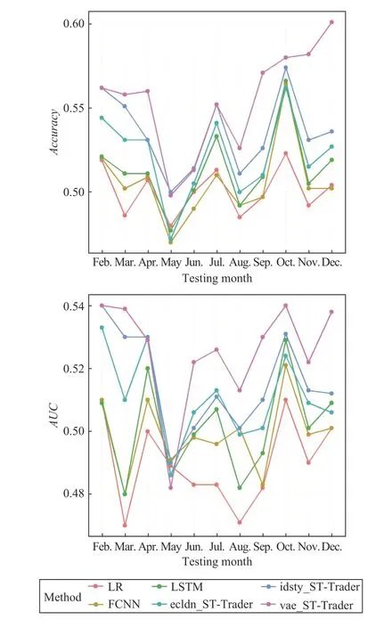
Fig. 3. ACC and AUC comparison for different methods across different testing months.

3) The Number of Neighbors to Communicate With: We compare performance of the proposed model on different granularity and different parameter K in Table III. We denote one-minute-interval and five-minute-interval price forecasting as ∆ t=1 and ∆ t=5. The superscript 1 and 5 highlight the best scores for ∆t=1 and ∆t=5. The results for ∆t=1 are aggregated across all testing months. There are two results worth mentioning. First, the outcomes of ∆ t=5 are better than∆t=1for all evaluation metrics. This result is as expected because the price movement of five-minute-interval is much less noisy than one-minute-interval due to a couple of reasons:i) Rare events like the flash crash can recover so quickly that five-minute-level data can almost screen out such events; ii)The recorded stock price is bounced back and forth between the bid and ask quote and the price fluctuation in five-minutelevel is less likely to be affected by the bid-ask bounce. If we have enough price observations on a longer interval, the predictive power of the proposed model can be expected toimprove.

TABLE III BINARY PRICE MOVEMENT PREDICTION WITH DIFFERENT PARAMETER K FOR ONE-MINUTE-INTERVAL AND FIVE-MINUTE-INTERVAL

Second, for the communication overhead parameter K,which is the number of nodes any target node i should exchange signals with in order to derive its local states, we use different K to explore how the communication affects the performance in different granularity. One-minute-interval achieves best performance when K=3 and five-minuteinterval achieves best performance when K=5, which means a finer granularity prefers a lighter communication to its neighbors. We give one possible explanation. For one-minuteinterval, where the fluctuation of price is more random, and hence the dependency is less reliable, the communication with more neighbors brings more noise in forecasting. While along with the time interval increasing, the price trend becomes more stable and the common fluctuation is more promising so that the infusion of neighborhood signals can be more informative. Thus, the number of neighbors for supporting the center node is a key hyperparameter to tune for a specific time-series forecasting task.

V. CONCLUSION

In this paper, we propose a spatial-temporal neural network framework GCN-LSTM, to utilize the spatial dependency or the latent interaction among firms in forecasting the stock price movement. The stock market has never been treated as a graph since there is not an inborn geographical location for stock entities. However, there is strong evidence that the interactions among firms affect the stock price movement.Experimental results show that our model outperforms other state-of-the-art methods on the real-world minute-level stock price data. Fundamental features represented in a spatial structure contribute to the forecasting accuracy improvement.For future directions, we plan to investigate how the combination of fundamental variables and fiscal reports,which can be seen as a dynamic cross-section assessment of a company, contributes to predicting the stock market trend.More practical time-series applications with potential spatial dependency should be explored under the proposed modeling framework. The advanced approaches [54], [55] to the fine tuning of hyper-parameters of the proposed framework should be explored.

ACKNOwLEDGMENT

The authors would like to thank Sophia Chen for proofreading.

APPENDIX

TABLE IV FIRM FUNDAMENTAL VARIABLES

TABLE V STOCK TICKER LIST

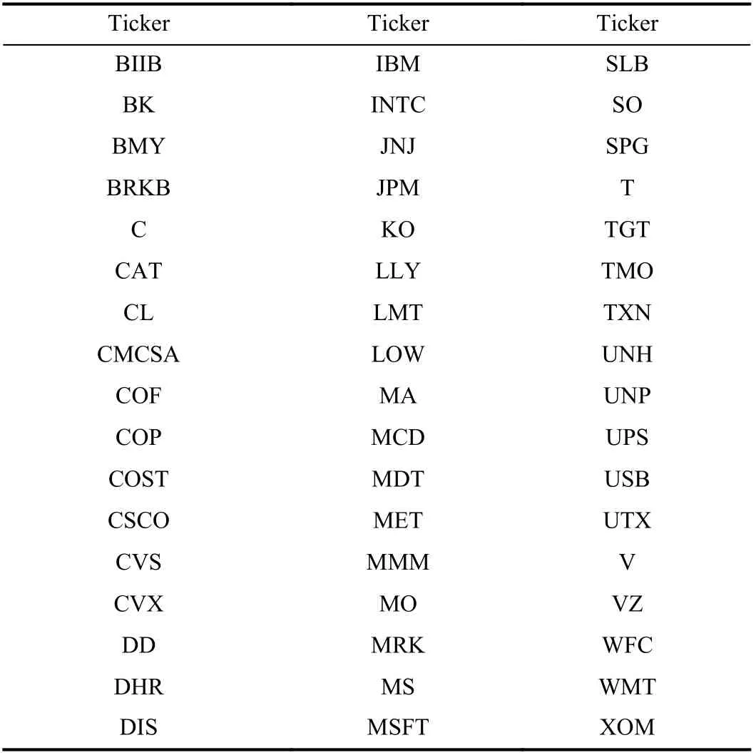
Table V (Continued)