Control of Non-Deterministic Systems With μ-Calculus Specifications Using Quotienting
2021-04-13SamikBasuandRatneshKumarFellowIEEE
Samik Basu and Ratnesh Kumar, Fellow, IEEE
Abstract—The supervisory control problem for discrete event system (DES) under control involves identifying the supervisor, if one exists, which, when synchronously composed with the DES,results in a system that conforms to the control specification. In this context, we consider a non-deterministic DES under complete observation and control specification expressed in action-based propositional μ-calculus. The key to our solution is the process of quotienting the control specification against the plan resulting in a new μ-calculus formula such that a model for the formula is the supervisor. Thus the task of control synthesis is reduced a problem of μ-calculus satisfiability. In contrast to the existing μcalculus quotienting-based techniques that are developed in deterministic setting, our quotienting rules can handle nondeterminism in the plant models. Another distinguishing feature of our technique is that while existing techniques use a separate μ-calculus formula to describe the controllability constraint (that uncontrollable events of plants are never disabled by a supervisor), we absorb this constraint as part of quotienting which allows us to directly capture more general state-dependent controllability constraints. Finally, we develop a tableau-based technique for verifying satisfiability of quotiented formula and model generation. The runtime for the technique is exponential in terms of the size of the plan and the control specification. A better complexity result that is polynomial to plant size and exponential to specification size is obtained when the controllability property is state-independent. A prototype implementation in a tabled logic programming language as well as some experimental results are presented.
I. INTRODUCTION
SUPERVISORY control problem was introduced in [1], [2]using deterministic automata representations of the plan and the control-specification. Since then several works focussed on generalization resulting from non-determinism in plants and from expressing control specification using temporal logics and bisimulation equivalences.
In the paper, we consider a DES supervisory control problem where a non-deterministic plant and specification are described as labeled transition systems and modal µ-calculus respectively. The central tenet of our technique is to develop a quotienting based technique to decide the existence of supervisor and generate the same if one exists. The quotienting technique can be described as follows. Given a plant P and the specification φ of the controlled plant,quotienting operation generates a new specificationψ=(φ/P)(in the same logic as φ) describing the obligation on supervisor C such that P when controlled by C satisfies φ. A supervisor C exists only and only when ψ=(φ/P) is satisfiable, and a model witnessing the satisfiability is one such C. The quotienting operation is defined on the basis of composition definition of P and C and the semantics of logic in which φ is defined (modal µ-calculus in our case). It also takes into consideration the possible non-determinism inP and controllability constraint of the possible supervisors (for example its inability to control/disable any uncontrollable actions of the plant).
The DES control problem subject to µ-calculus specification was examined in [3], where the problem was considered in the setting of control of a deterministic plant. The authors also allowed time-varying uncontrollable actions and “projectiontype” partial observation function. The work was later extended by considering indistinguishable actions in [4], [5].We allow nondeterminism in the plant model and more general state-based uncontrollable events under complete observability of events. While at its core our technique also relies on reducing the problem of supervisor synthesis to that of model generation for a satisfiable formula, there are several significant differences; the key distinguishing aspects are enumerated as follows:
1) We perform quotienting at the level of µ-calculus formulas. On the other hand, [3]–[5] computes the alternating tree automata representation of µ-calculus and apply quotienting on the tree automata.
2) Quotienting lets us handle not only state-dependent controllability requirements but also nondeterministic plants in a straightforward manner. In contrast, [3]–[5] impose a controllability constraint as a separate µ-calculus formula,which is state-independent.
3) In [3]–[5], a plant model is assumed deterministic, and further the controllability constraint used assumes a supervisor to be deterministic, obviating the need for the µ-calculus framework. Our work is based on our prior conference publication [6] and allows nondeterminism in plant as well as controller models. Also, while [3]–[5] allow a partial observability of events, this is not adequate to capture nondeterminism: Partial observation identifies only the actions from the point of observation, whereas nondeterminism identifies actions as well as control and specification from the point of observation. Reference [7] proposed extension to their prior work [3] to incorporate nondeterminism in both plant and controller models; in [8] we proposed extension to our prior work [6] to incorporate partial observability.
References [9], [10] also considered automata-theoretic quotienting. However, as opposed to satisfiability checking for supervisor synthesis, the authors coupled the existence of supervisor with the specification logic expressed in quantifiedµ-calculus. Furthermore, as with [3], the work in [10] is limited to deterministic plants.
Our quotienting procedure is closely related to the one described in partial model checker [11]. The work presents quotienting operation on equational µ-calculus against labeled transition systems. The main aim is to show the applicability of quotienting for model checking systems with regular structures (e.g., ring topology). This work is generalized in[12]wherequotientingisdefinedfor µ-calculusformulas against arbitraryCCSprocesses.The techniqueis coupled with limit computation over sequence of µ-calculus formulas to develop a method for model checking parametrized systems. We present a quotienting operation for labeled transition representing a non-deterministic plant model where labels capture plan-events and certain events are classified as controllable.
The result of quotienting operation is a new µ-calculus formula such that its satisfiability proves the existence of a supervisor and the satisfiable model is one such supervisor. A number of notable work have presented different techniques for satisfiability checking for µ-calculus by verifying alternating tree automata emptiness [13], by identifying winning strategy in parity games [3], [14], [15], or verifying satisfiability of equivalent disjunctive µ-calculus formula. In contrast, we use a tableau-based method for satisfiability checking and model discovery. Central to our tableau is the maintenance of a history set which ensures that least fixed point sub-formulas are captured by finite-path in the satisfiable model while greatest fixed point sub-formulas are captured by cycles in the model.
The contributions of this work is summarized as follows:
1) We present a quotienting technique for control synthesis,where the desired property is expressed in µ-calculus, and a plant model is expressed as finite state machine. The proposed quotienting technique methodically translates the desired property expressed in µ-calculus into obligation for a controller, that is also expressed in µ-calculus. This allows us to deal with non-determinism in plant model and statedependent controllability directly using the quotienting.
2) We have generalized existing quotienting technique used in the context of partial/compositional model checking. Unlike model checking, where all events are of the same type, in our case, events can be classified as controllable vs.uncontrollable, and which can vary from state to state.
3) We present a tableau-based technique for generating satisfiable model (which, in our case, is the model of a controller) for µ-calculus formula.
4) We present a preliminary implementation to show the viability of our technique.
The rest of the paper is organized as follows. In Section II,we discuss the relevance of our work in the context of controller synthesis work that uses techniques other than quotienting. Section III gives a brief overview of the modal µ-calculus (Section III-B), followed by the description of the control problem (Section III-C). Section IV presents a simple example that is used for illustrating our approach. In Section V we present our technique of quotienting µ-calculus specification with respect to a plant model to obtain a quotiented formula representing the obligations of a supervisor. We then develop a methodology to check for the satisfiability of a quotiented formula and identify a supervisor model when possible (Section VI). Section VII describes our prototype implementation. Preliminary experimental results are discussed in Section VIII. We conclude the paper in Section IX.
II. OTHER RELATED WORK
The control problem in domain of nondeterministic plant and specification is studied in [16]–[20]. The authors in [20]show how to transform their control problem in nondeterministic setting to one in deterministic setting with an added partial observability. Control of plants modeled using nondeterministic state machines for language specification is also studied in [21], [22]. All the work used deterministic supervisors.
The use of a nondeterministic supervisors for specification represented using language model was explored in [23], [24].The problem of nondeterministic control was formalized in[25]. The authors focused on control under partial observation for language specification and introduced the notion of achievability (a property weaker than controllability and observability combined). Nondeterministic supervisors have also been used in works allowing nondeterminism in specification. Such specifications are able to impose both sequencing and branching constraints and are modeled using branching-time temporal logic such as CTL∗and µ-calculus,or using bisimulation or simulation equivalence type requirements. In [26] a nondeterministic specification was specified in the temporal logic of CTL∗, generalizing the work reported in [27] which used CTL to express specification.Other work related to control subject to temporal logic based specification include [3], [28]–[31].
Bisimulation relation has been used as a technique for supervisory control of deterministic systems subject to language specifications in [32]–[36] the controllability and observability are characterized as a bisimulation type relation.Reference [37] studied the bisimilarity control for a deterministic specification, treating all events controllable.Reference [38] studied bisimilarity control for a partial specification (defined over an “external event set”) under several restrictions: Deterministic plant, all events controllable, and all events treated indistinguishable from the specification perspective be either all enabled or all disabled at a state. Reference [39] studied the bisimilarity control for again deterministic plants subject to a possibly nondeterministic partial specification, thereby relaxing some of the assumptions of [38].
The most general bisimulation equivalence control problem was finally studied in [40], in which both the plant as well as the specification are nondeterministic. (The same authors also studied the special case of deterministic control in [41], and provided additional comments in [42].) In [43], the author presented a new bisimulation based control synthesis technique with an improved runtime complexity. The extension to allow partial observation of events was reported by the same authors in [44], [45], and the simulation equivalence control under the above generalized framework was addressed by the same authors in [46]. [47] discussed synthesis of maximally permissive controller in the context of simulation equivalence.
In our technique, as we focus on satisfiability of properties expressed in μ-calculus, it is equivalent to synthesis problem where the controlled plant is bisimulation equivalent to the desired behavior. Furthermore, our quotienting based technique does not guarantee the generation of maximally permissive controller. However, note that the behavior of the controller (being synthesized) is expressed in μ-calculus formula resulting from quotienting. In other words, all feasible controller behavior, including the maximally permissive one,is captured by the μ-calculus formula. As part of future work,it would be interesting to investigate and extend our tableaubased model generation technique to generate a maximally permissive controller, and also explore the application of BDD representation (as for example in [48]) for computational improvement.
III. PRELIMINARIES
A. Labeled Transition System
The dynamic behavior of system is typically expressed using transition system, where states in the system correspond to configurations of the system, while the directed edges/transitions between configurations describe the evolution of the system. In our case, we augment each transition with label to capture the event/action-name that identifies the evolution due to the transition. Formally, a labeled transition system (LTS) M is (S,A,T,AP,L), whereS is the set of states, T ⊆S×A×S is the set of transitions labeled by actions in A and L:S →2APis the labeling function which maps states to sets of propositions. If a state is“labeled” by a set of propositions, we say that the propositions are valid or true in that state; all other propositions are false in that state. The truth-values of the propositions describe the states.
B. Propositional µ-Calculus Specifications
The µ-calculus [49], [50] uses explicit least and greatest fixed points to express temporal ordering of events and states.The set of properties, thus, induced is strictly larger than the one expressible in temporal logics such as LTL, CTL. The syntax of µ-calculus formulas involves propositional constants( tt, ff) , atomic propositions AP, modal actions A with modalities ([] and DIAM ), boolean connectives ( ¬, ∨, ∧),fixed point variables X ∈X and expressions.

In the above, 〈a〉 is referred to as diamond modality over action a; informally, it expresses the existential quantification a successor. On the other hand, [a] is referred to as box modality over action a; informally, it expresses the universal quantification of all a successor. The fixed point formula expression σX.ϕ includes the type of fixed point σ ∈{µ,ν} (µ:least fixed point operator and ν: greatest fixed point operator),the variable X bound by the operator σ, and ϕ the formula describing the definition of the fixed point expression. In any formula, a variable not bound by any fixed point operator is called free variable. The set of all µ-calculus formulas defined over the domain (AP,X,A) is denoted Φ[AP,X,A]. For a formula φ, we will use the following notational convenience:FV(φ) denotes its set of free-variables, S ub(φ) denotes its set of sub-formulas, |φ|, called length of φ, denotes the number of boolean and modal operators in φ, and ad(φ), called alternation depth of φ, denotes the number of nesting betweenµ and ν in φ [51]. a d(φ) is recursively defined as follows:


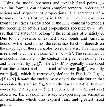


Fig. 1. Semantics of µ-calculus formula.
where for σX.φ, fp(X)=σ . We use nd(φ) to denote the nesting depth, i.e., the number of nestings of fixed point expressions in φ. The definition is identical to that forad(φ)except when φ =σX.φ.another initialized LTS. Note that P and C share the sets of actions ( A) and atomic propositions ( AP). The controlled plant is obtained by the strict synchronous composition of P and C,denoted by P||C, which is defined as:(SPC,A,δP||C,AP,LP||C,S0,PC) , where SPC=SP×SCis the state set; A and AP are the same sets as given in P ; δP||C⊆SPC×A×SPCis the set of transitions of P||C and is given by

We use LTSs to represent the discrete event systems (DES)expressing the plant model and the supervisor expressing the controller. Some subset of these LTSs are referred to as the initial or start states capturing the initial configurations of the plant and the supervisor. We will refer to these LTSs as initialized LTSs. An initialized LTS is satisfy a propertyφ expressed in µ-calculus if and only all initial states of the LTS belong to the semantics of φ.
C. Supervisory Control
An uncontrolled discrete event plant P is modeled as an initialized LTS, P=(SP,A,δP,AP,LP,S0,P), whereSP,A,δP,AP , and LPhave the usual semantics. We use S0,P⊆SPto denote the set of start or initial states of the plant. Note that transitions from states can be controllable or uncontrollable.Hence, for each state s, the actions on the outgoing transitions are partitioned into two groups: the controllable action set Ac(s), and the uncontrollable action set Au(s).
A supervisor C=(SC,A,δC,AP,LC,S0,C), is defined as

The synchronous composition induces the control imposed by the supervisor on the plant. For instance, a composed state(s,q)has an outgoing transition on an action only when the both the supervisor and the plan has the outgoing transition on the same action; otherwise, the transition is absent. That is, if a supervisor at the state q wants to disallow a transition with action a from the state s, then it simply does not have any evolution on action a. However, note that a supervisor cannot disallow any the uncontrollable actions in plant. In other words, if a is an uncontrollable action from state s and the supervisor state composed with s is q, then q is required to have an evolution on the action a. This requirement is referred to as the control compatibility.
IV. ILLUSTRATIVE ExAMPLE
We illustrate the salient features of our technique using a simple but representative problem involving controlling the moves of a cat and mouse in a maze Fig. 2(a). The maze consists of several numbered rooms, which are connected by passage-ways/doorways—some accessible by the mouse (denoted by mi) and some others accessible by the cat (denoted by ci). All doorways have directionality and all, except c7are controllable. The objective is to generate a controller which appropriately controls (closes) the controllable doorways such that the cat and mouse (initially placed in rooms 2 and 4,respectively) never occupies the same room. The possible(unrestricted) movements of the cat and the mouse (Fig. 3)can be obtained by the asynchronous composition of the movements of the cat with the movements of the mouse (Fig. 2(b)),modeled as labeled transition systems. The nodes in the transition system denotes the rooms in which the entity resides and the directed-labeled edges denotes the movement of the entity from the source node/room to a destinate node/room via the doorway represented by the labels. The movements of the cat and the mouse forms the plant model, which in this example is non-deterministic as the cat can nondeterministically choose to move from room 0 to either room 1 or 3 via doorway c1. As noted before, the supervisor is required to control the movement of the cat and the mouse such that they do not occupy the same room simultaneously.This requirement can be expressed in µ-calculus as νX.(p∧[−]X), where p represents a proposition which is true only when the cat and the mouse are not in the same room.We use a short-hand notation [−] to represent any action. The greatest fixed point formula represents the states wherep holds and this continues to remain true after any action.

Fig. 2. (a) Cat-Mouse maze; (b) Cat-Mouse models.
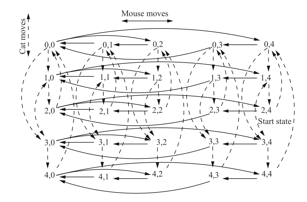
Fig. 3. Plant model for Cat-Mouse example in Fig. 2(b).
The above can be viewed as safety requirement of the supervisor objective. The requirement can be further augmented to include liveness requirement that the cat and mouse is always able to return to their start state. This can be expressed using alternating fixed point formula:νY.(µZ.(q∨〈−〉Z)∧p∧[−]Y), where p has the usual meaning and q represents a proposition which is true only when the cat and the mouse are at their respective start states (i.e., the cat is in room 2 and the mouse is in room 4). The greatest fixed point formula over the variable Y has a nested least fixed point formula over the variable Z. The least fixed point formula represents the states which can eventually reach the start state while the outer greatest fixed point formula ensures that the cat and the mouse are never in the same room.
V. QUOTIENTING µ-CALCULUS SPECIFICATIONS
We present here a formal description of the problem at hand. Given a DES P and a desired controlled behavior φ◦of P expressed in µ-calculus, the problem is to

where C denotes a control-comptabile supervisor,P||C denotes the composition of the plant with the supervisor, and|=denote the relationship where the left-hand side is a satisfiable model for the property in the right-hand side. In other words, does there exist some supervisor under the presence of which the plan satisfies the desired behavior.
We reduce this problem as follows. The obligation onP||C is to satisfy φ◦. We transform that obligation to an obligation on on C; we refer to this new obligation as φ÷. The transformation is such that

That is, satisfiability of the desired behavior by a controlled plan is reduced to the satisfiability of a new behavior by the supervisor alone. In other words, the plant is controllable(supervisor exists) to conform to desired behavior if and only if the transformed formula φ÷is satisfiable. This not only addresses the problem of whether a supervisor exists but also presents a roadway to generate a supervisor, if one exists. The satisfiable model for φ÷is one such supervisor.


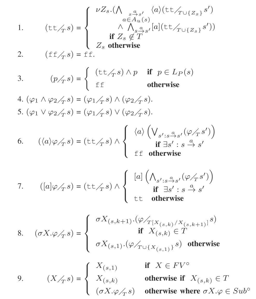
Fig. 4. Quotienting rules.
As true is satisfied in any plant state s , Rule 1 in Fig. 4 captures that any supervisor state q composed withs necessarily satisfies the control compatibility requirement.That is, for any uncontrollable action a ∈Au(s) from s to s′,there is “matching” action from q and the destination state(e.g., q′) satisfies the control compatibility requirement in the context of the state s′. This is represented by the conjunction of 〈a〉 modal formula (a ∈Au(s)). On the other hand, actions that are not in Au(s) may or may not be allowed by the supervisor. This is captured by the box-modality formula.Recall that the box-modality can be satisfied in the absence of the modal action. Finally, note that the result of quotienting is a greatest fixed point formula over a new variable Zs. The tag set records that the formula tt is quotiented against s. The quotienting operation is recursive; the recursion terminates when tt is quotiented against s more than one time, and the result is equal to the corresponding fixed point variable Zsas recorded in the tag set.


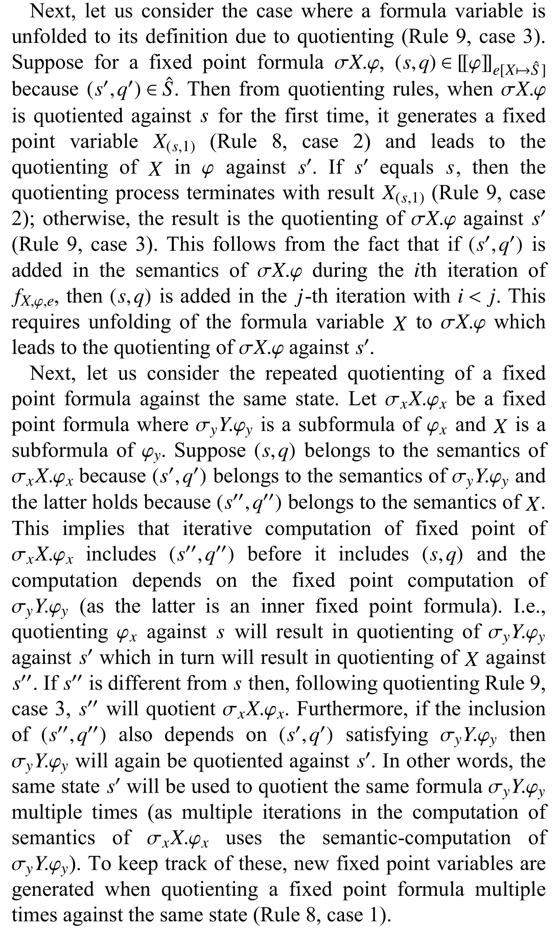
Rules 8 and 9 are used for quotienting fixed point formula and fixed-point variable respectively. Due to i) the multiplicity of the plant states, ii) the nesting of fixed point formulas, and iii) the fact that quotienting is performed by recursively descending the parse-tree of the sub-formulas, the quotienting of a fixed point formula can occur in association with different states and multiple times with each state. The tag set keeps track for each fixed-point formula, and for each state, the number of times the fixed-point formula has been quotiented (with respect to the state). The count is incremented by one each time such a quotienting is performed. We argue that the count remains bounded. As a result the size of tag set itself remains bounded, and we provide a value for such a bound (see Theorem 1).
Rule 8 states that the quotient of a fixed point formula is the fixed point of the quotient formula, where the fixed point variable X(s,j)captures three features:
1) the variable X that is bound by the fixed point in the formula being quotiented;
2) the state s that is used to quotient the formula;
3) the number of times the formula is quotiented by s. This value is incremented appropriately by keeping track of the previous count in the tag set T.

As fX,φ,eis monotonic, the function (f/s)X,φ,eis also monotonic for all s. Therefore, quotienting a least (greatest)fixed point formula results in another least (greatest) fixed point formula. As such, the quotienting Rules 8 and 9 do not alter the fixed point nature of the formula being quotiented.

Fig. 5. Snippet showing application of Rules 7–9 of Fig. 4.

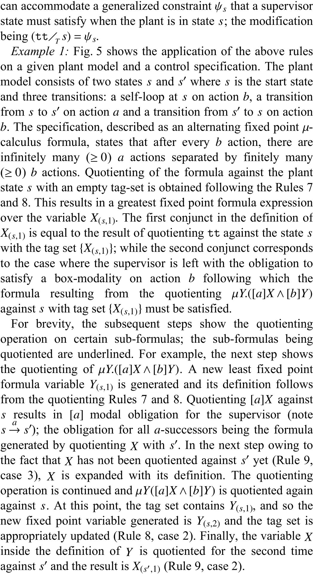
Example 2: Fig. 6 shows the quotienting of the control specification of Section IV against two of the states of the catmouse plant model. The figure also presents quotienting oftt against a plant state. The plant states are of the formsijrepresenting the state when the cat is in room i and the mouse is in room j. Proposition p is true in the states sijwith i ≠j.Fig. 7 shows the recursions of the quotienting operations. For brevity, we have omitted the tag-sets and the formula expressions for the control-compatibility. The node enclosed within a square box denotes the termination of quotienting, for the reason that the definition of X has already been quotiented against s34(Rule 9, case 2).
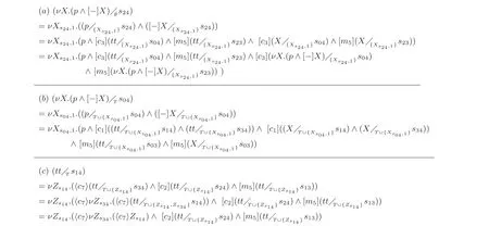
Fig. 6. ν X.(p∧[−]X) quotiented against (a) s24 and (b) s04 (with non-determinism on c1) ; (c) tt quotiented against s14.
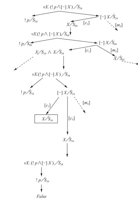
Fig. 7. Quotienting recursion snapshot in Cat-Mouse model.
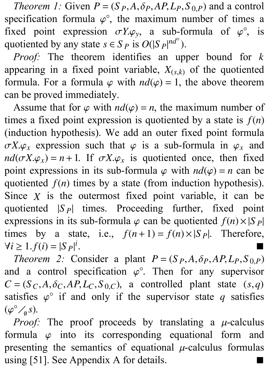
We have the following theorems establishing the termination of the quotienting of a fixed-point formula and the correctness of the reduction of the control problem to the satisfiability of the quotiented formula.
VI. SATISFIABILITY CHECKING AND MODEL DISCOVERY
In this section, we focus on verifying the satisfiability of µ-calculus formula φ⋄∈Φ[AP,X,A]. If the formula is satisfiable,we also develop a model witnessing the satisfiability. This technique will be used to generate/identify the supervisor.
Preliminaries: Recall that, the µ-calculus formula expresses temporal ordering using explicit greatest and least fixed points, and these fixed point sub-formulas can have arbitrary nesting. We assign identifiers to each fixed point variable based on their binding and nesting depth.

The id of greatest fixed point variables are even, while the id of least fixed point variables are odd. The id of the variable bound by the outer-most fixed point is the largest.
A. Tableau-Based Approach
We present a set of implications, which if valid, establishes not only the satisfiability of the µ-calculus formula but also helps identify a satisfiable model. These implications form a tableau written as

i.e., A1∧A2∧...An⇒A. In other words, in order to prove the validity of A, we need to verify the validility of A1,A2,...,An. Given a obligation to prove some claim A, the tableau induces a proof-tree, where the nodes in the tree represents the obligations and sub-obligations (nemerator and denominators of the tableau rule) and edges represent the dependency (conjunctive). A proof tree successfully validates a claim (at its root) if all its leaf nodes are valid.
In our setting, each tableau rule is of the form


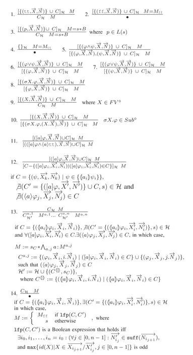
Fig. 8. Tableau for satisfiability and model discovery for φ ⋄.
Discussion: If the objective is to verify the satisfiability of φ⋄, a tableau-tree is constructed rooted at the node“{(φ⋄,ϵ,ϵ)}∅M”. The children of the root are identified by“firing” the tableau-rule whose numerator matches with the root. This firing may result in multiple new nodes in the tableau tree, and each of these new nodes may lead to new nodes by firing new tableau-rules. Note no successor is created for a tableau-rule whose denominator is empty(denoted as a “ •”). When a tableau-node does not have any children (leaf-node), the model associated with that tableaunode is assigned a concrete value; and this results in a path in the model expression starting from the root of the tableau to the leaf-node. Once the iterative tableau-node creation terminates along all branches of the tableau tree, the root node gets associated with a concrete model. At this point, the formula at the root, φ⋄, is satisfiable if and only if the model expression M of the root node is not Mff(see Theorem 3).
Note that, the set C correspond to conjunction of formula.As a result Rule 1 states that if one of the conjuncts is tt, then obligation is to satisfy the rest of the conjuncts. On the other hand, Rule 2 states that only a false model Mffcan witness the satisfiability of a conjunctive formula where one of the conjuncts is ff.

Rule 4 captures the scenario where there is no obligation for proving satisfiability and therefore, the true model (or any model) can be used as a witness.
Rules 5–7 deal with conjunctive and disjunctive formula.Note that Rules 6 and 7 result in two different tableau-tree depending on the consideration of left- or right-conjunct.
Rule 8 states that M satisfies a fixed point formula σX.φ if and only if it satisfies φ. Rule 9 corresponds the scenario where one of the conjuncts is a free variable. As any suitable mapping of free variables to sets of states (for non-false models) can be generated, the denominator of the tableau rule simply discards the free variable. In typical scenario, formulas will not involve free variables (all variables will be bound by some fixed point expression).

Rules 11–14 apply when all the formula expressions in the numerator C are modal formula expressions. Rules 11 and 12 are applied when there exists a box-modal formula on an action a with no diamond-modal formula on the same action.Recall that, there are two ways to satisfy a box-modal formula[a]φ . Either every a transition leads to destinations that satisfy φ, or there is no a transition. Accordingly, Rule 11 captures the first scenario; and Rule 12 considers the second scenario.Note that, in Rule 12 all box-modal formula on the same boxmodal actions are removed from the formula set in the denominator.
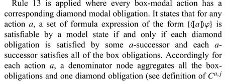
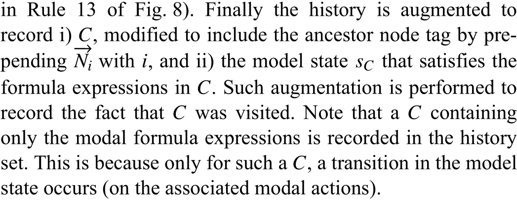
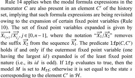
Example 3: Table I presents the snapshot of the tableau for identifying a model satisfying the formula: ν X.µY.([a]X ∧[b]Y).The formula expressions at node A1 in the tableau are the same as the formula expressions at node A0. The formulas at A1 originated from the formula [a]X at A0 (see history set at A1). The outermost fixed point variable expanded between these tableau-nodes is X, the greatest fixed point variable. As the such the model state at node A1 is the same as the model state at node A0, namely state s.

TABLE I SNAPSHOT OF A TABLEAU
Theorem 3: Given a µ-calculus formula φ⋄, it is satisfiable if and only if there exists a tableau with root node“{(φ⋄,ϵ,ϵ)}∅M ”, such that M is assigned to a non falsemodel.
Proof: The completeness of our satisfiability checking follows from the fact there is one tableau rule for each syntactic construct of a µ-calculus formula. Then to show the soundness of our satisfiability check it suffices to show the soundness of each of the tableau rules. The soundness of the tableau rules follows from the semantics of the µ-calculus formula (Fig. 1). The soundness of the Rules 1–13 can be realized directly from the discussions given preceding the theorem statement.
The soundness of Rule 14 is more involved as it depends on the semantics of fixed points. Consider first the semantics of a least fixed point formula µX.φ, which is the smallest state-set satisfying φ. A least fixed point formula µX.φ is satisfiable if and only if [[φ]]e[X■→∅]is non-empty. In other words, µX.φ is satisfiable if and only if the model for φ is a non false-model when the model corresponding to X inside φ is Mff. Rule 14 in the tableau captures precisely this fact and states that if the outermost formula variable expanded in a tableau starting and ending in the same tableau node is a least fixed point variable,then model corresponding to the later node is a false-model. A dual property holds for νX.φ, namely the formula is unsatisfiable if and only if [ [φ]]e[X■→S]is empty.

Note that when the controllability constraint is stateindependent, Rule 1 can be simplified as

VII. IMPLEMENTATION
A prototype implementation for performing the quotient operation and for checking satisfiability and identifying a supervisor model has been realized in XSB, a tabled logic programming language [54]. The tabling feature in XSB is used to avoid repeated subcomputation in addition to computing the least model of normal logic programs Predicates or relations are defined as logical rules in XSB in the following manner:

The predicate Goal evaluates to true only when each of the subgoals in the right-hand side of “:-” evaluates to true. In essence, the above logical rule represents

A rule with empty right-hand side is referred to as a fact.
XSB Encoding of DES Problem: Models in supervisory control problem, represented as labeled transition systems, are encoded by rules and facts in XSB:
1) ctrans(S, A, T), denotes a transition of a component in a plant model from a state S to a state T via an action A,
2) trans(S, A, T), denotes a transition from a plant state Sto a plant state T via an action A,
3) startstate(S), denotes the fact that S is a start state of the considered plant model,
4) label(S, P), denotes the labeling of a plant state S with a proposition P.
5) uncontrollable(S, AList), states that the actions in AList are not controllable at a state S.
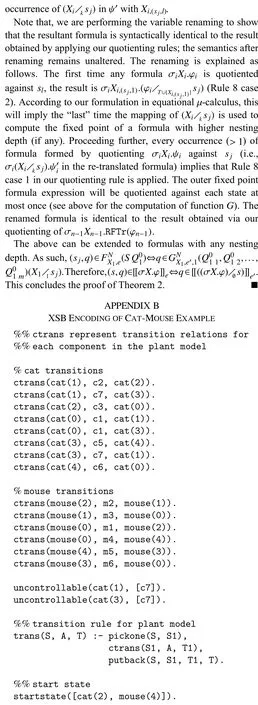
The encoding of the models for the cat-mouse example (Fig. 2)is shown in Appendix B.
The plant model is defined by the product of its components, i.e., a transition in plant model corresponds to a transition in one of the participating components. A state in a plant model is represented as a list of component states.Appendix B shows the encoding of the transitions of the plant model derived from the encoding of the transitions in its components. The predicate pickone selects a component state S1 from the plant state S. For a transition on an action A, the destination plant-state T is reconstructed form the destination component-state T1 using the predicate putback. The start state of the plant is encoded as a fact that initially the cat and the mouse are in rooms 2 and 4 of the maze respectively.
Formula definition is represented by a term fDef with three arguments representing the fixed point variable, fixed point operator and the body of the definition. For example, the formula ν X.(p∧[−]X) is represented as

In the above, the terms and and fBox are used to capture the boolean connective ∧ and box modal operator[]respectively. Similar terms ( or and fDiam) are used for capturing the dual operators. The term prop is used to denote the atomic propositions. Finally, “_” infBox(_,form(x))represents any action.

The following shows a snapshot of compiling and executing the quotienting program in XSB:

In the above, quot is the main program file which contains the quotienting rules and the directives to include the plant model file (e.g., catmouse.P containing the model for the plant). The result of quotienting is obtained via grounding of variable QRes which holds the valuation of the outermost fixed point variable of the quotient. The actual formula expressions are asserted as facts and can be viewed using“listing(fDef)”.

The predicategenmodel(SetOfFormula,History,Model)represents the tableau node CHM in Fig. 8, where SetOfFormula represents C , and History andModel represent the associated history set H and the modelM respectively.
For details of implementation and tool documentation see http://www.cs.iastate.edu/~sbasu/control-quot.
A. Formula Simplification
Formula generated via quotienting can be prohibitively large. We use a number of simplification rules following the semantics of the µ-calculus formula expressions, that reduces the length of the generated formula. The simplification rules are as follows:

B. Model Simplification
The models generated using tableau rules can be simplified by merging bisimilar states in the model. Bisimulation equivalence [55] states that two states s1and s2are equivalent if they are related by the largest bisimilarity relation R defined as follows:

VIII. ExPERIMENTAL RESULT
We revisit the cat-mouse example from Section IV. The specification formula νX.(p∧[−]X) is quotiented against the plant model and the tableau-based model discovery algorithm is applied on the quotiented formula to obtain a candidate supervisor. The supervisor model we obtained is presented in Fig. 9(a). In the figure, the states in the supervisor represent the corresponding rooms in which the cat and the mouse are present. Note that, when the cat and the mouse are in rooms 0 and 4 respectively, the supervisor can allow the cat-move c1.As this is a non-deterministic transition for the cat, the successor supervisor state designates that the cat can be either in room 1 or 3.

Fig. 9. Supervisors for plant in Fig. 2 for specifications (a)νX.(p∧[−]X)and (b) ν Y.(µZ.(q∨〈−〉Z)∧p∧[−]Y).
For finding a supervisor for the more general specification νY.(µZ.(q∨〈−〉Z)∧p∧[−]Y), we quotiented the formula against the plant model and using the tableau-based model discovery algorithm to obtain a supervisor (Fig. 9(b)), which can be seen to be less permissive than the previous one, as expected. Since the specification demands that the controlled plant must ensure that the start state is always reachable, the supervisor disallows the transitions m5and c3from the states(0,4) and (2,3) respectively; these transitions lead the controlled plant to the deadlocked state (0,3) from where the start state ( 2,4) is unreachable.
Fig. 10(a) presents the deterministic plant obtained by renaming the cat-move from 0 to 3 by c4. The supervisor corresponding to the specification νX.(p∧[−]X) is presented in Fig. 10(b). In this case, the supervisor can distinguish between the two states, one where the cat and the mouse are in rooms 1 and 4 respectively and the other where the cat and the mouse are in rooms 3 and 4 respectively. In contrast to the nondeterministic case where these states were reached on the single cat-move c1, the determinization results in the reachability of the states via two distinct cat-moves c1and c4.
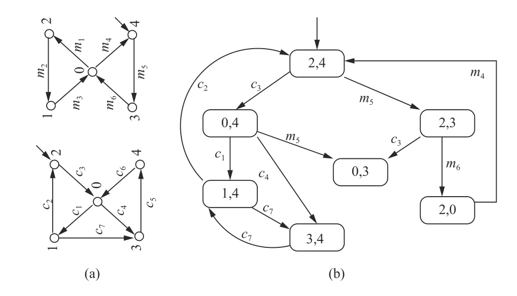
Fig. 10. (a) Deterministic cat and mouse models and (b) Supervisor for specification ν X.(p∧[−]X).
Table II summarizes the effect of applying the simplification rules (see Section VII) in both quotienting and model discovery modules of our implementation for both the nondeterministic and deterministic models. For example, in the absence of simplification, for the control specification νX.(p∧[−]X), quotienting generates a formula expression consisting of 341 fixed point sub-formulas, while the simplification reduces it to one consisting of only 10. Tableaubased model discovery with no simplification identifies a model containing 26 transitions for the simplified quotiented formula (possessing 10 fixed point formula expressions).Bisimulation equivalence reduces the number of transitions to 9. The entries “−” represent the case where the execution is terminated after quotienting generated more than 3000 subformulas.
IX. CONCLUSION
We presented a technique for supervisory control of nondeterministic discrete event plants under complete observation of events subject to specification expressed in the propositional µ-calculus. Central to our method is a directquotienting of the µ-calculus specification against the plant model. A control-compatible supervisor exists if and only if the quotiented formula is satisfiable, and further a model witnessing the satisfiability can be used as a supervisor. We also developed a sound and complete tableau-based methodology for satisfiability checking and model discovery of µ-calculus formulas. Our technique works for nondeterministic plant models and can generate supervisors that are also nondeterministic. The complexity of verification and synthesis is single exponential in the size of the plant as well as the specification. A prior work on control for bisimilarity [40] has a complexity that is doubly exponential in the size of the plant and the specification.
Some of the future avenues for research include incorporating the notion of partial observability of actions into quotienting.
APPENDIx A PROOF FOR THEOREM 2
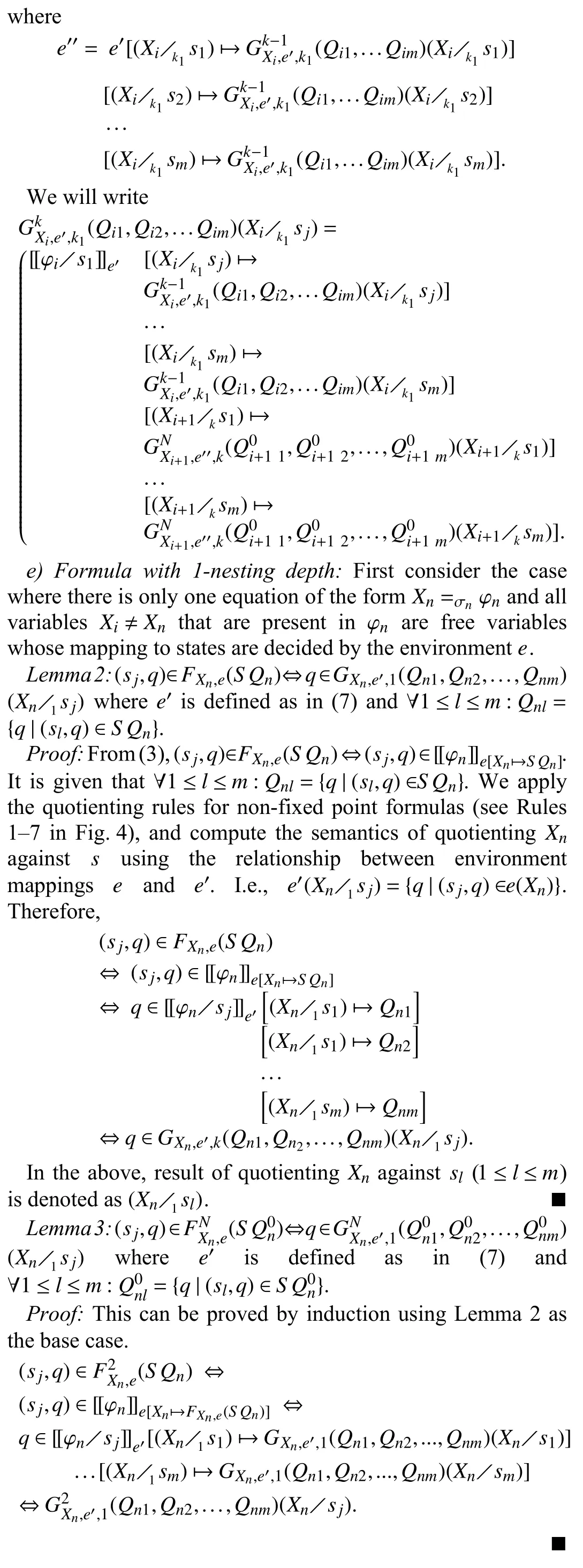
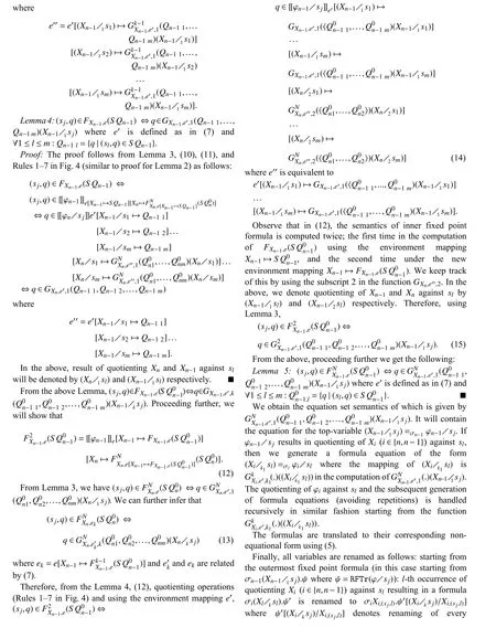
a) Equational µ-calculus: Equational system of µ-calculus consists of a set of equations of the form X=σϕ whereX belongs to the set of the fixed point variables and ϕ belongs to the set of basic formulas defined by the following syntax:
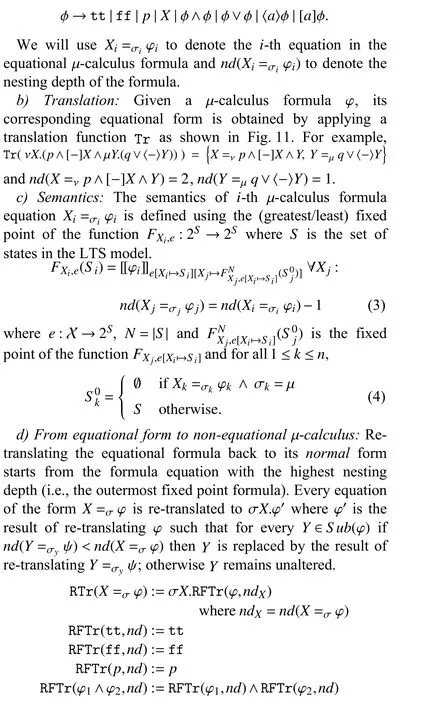

TABLE II RESULTS FOR CAT-MOUSE ExAMPLE
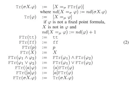
Fig. 11. Translating µ-calculus to its equational form.
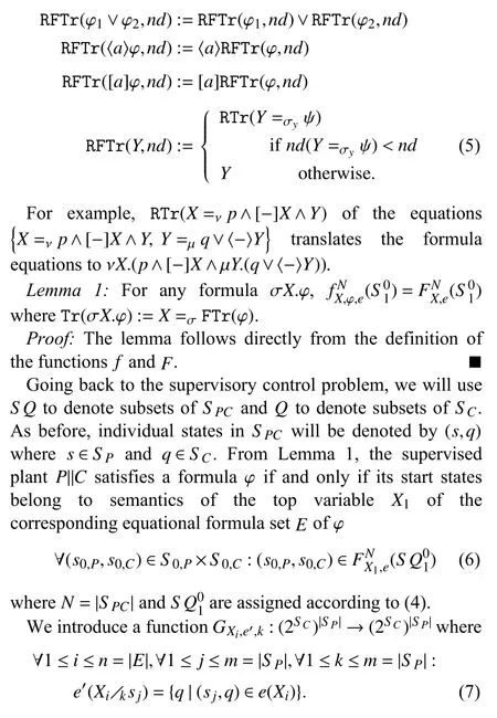
The function is defined as follows:

1


杂志排行
IEEE/CAA Journal of Automatica Sinica的其它文章
- Review of Research and Development of Supernumerary Robotic Limbs
- Decentralized Dynamic Event-Triggered Communication and Active Suspension Control of In-Wheel Motor Driven Electric Vehicles with Dynamic Damping
- ST-Trader: A Spatial-Temporal Deep Neural Network for Modeling Stock Market Movement
- Total Variation Constrained Non-Negative Matrix Factorization for Medical Image Registration
- Sampled-Data Asynchronous Fuzzy Output Feedback Control for Active Suspension Systems in Restricted Frequency Domain
- Predicting Lung Cancers Using Epidemiological Data: A Generative-Discriminative Framework
