Approach for Grid Connected PV Management:Advance Solar Prediction and Enhancement of Voltage Stability Margin Using FACTS Device
2021-01-23MdMasumHowladerAzizUnNurlbnSaifMDShahrukhAdnanKhanMahfujHowladerMohammadRokonuzzamanMdTanbhirHoq
Md.Masum Howlader | Aziz Un Nur lbn Saif | MD Shahrukh Adnan Khan | Mahfuj Howlader | Mohammad Rokonuzzaman | Md Tanbhir Hoq
Abstract—The uncertainty in solar energy is different from conventional, dispatchable generation fuels and difficult to incorporate into the standard system operating procedures.In the first part of this work, the machine learning algorithm is used to train models based on solar irradiance data and different meteorological weather information to predict the solar irradiance for different cities to validate the forecasting model.Again, the intermittent and inertialess nature of photovoltaic (PV) systems can produce significant power oscillations that can cause significant problems with dynamic stability of the power system and also limit the penetration capacity of PV into the grid.In the second part, it is shown that the residue-based power oscillation damping (POD) controller obviously improves the inter-area oscillation damping.The validity and effectiveness of the proposed controller are demonstrated on the three-machine two-area test system that combines the conventional synchronous generator and flexible alternating current transmission systems (FACTS) device using simulations.This report overall puts an in-depth analysis with regard to the challenges of solar resources with integrating, planning, operating, and particularly the stability of the rest of the power grid, including existing generation resources, customer requirements, and the transmission system itself that will lead to an improved decision making in resource allocations and grid stability.
1.lntroduction
The transition towards sustainable energy supply, mainly, with the increasing contribution of photovoltaic (PV) to the distribution grid, has significant impacts on the transmission and distribution of electricity supply systems.Power received from renewable energy (RE) systems exhibits fundamentally different generation behaviors compared with the traditional energy sources, such as fossil fuels.The power generation from conventional sources can easily be met exactly with the given electricity demand, while the availability of solar and wind energy is mostly determined by the prevailing weather conditions and is therefore highly inconsistent.To effectively manage energy systems with integrated renewable sources, it is important to have clear information about the availability of solar irradiation and its variability.One of the main concerns for utility operators and grid system managements is the supply variability for renewables caused by the transient weather conditions which could have a significant impact on the whole energy supply system.For example, overestimating reserve requirements may result in an unnecessary expenditure of capital and higher operating costs.This variable nature constitutes the major challenge for the integration of renewables into the power supply network and thus the implementation of new methods for balancing the supply and demand is required[1].
Solar energy generation systems are highly dependent on the local, site-specific condition, such as the shading and local weather condition which makes it difficult to determine the solar irradiance, and consequently electric power[2],[3].The variability of RE creates a major challenge for the integration of RE into the energy supply system and urges for devising new methods of balancing the supply and demand[4],.In our previous work, we designed a prediction system based on the machine learning approach to forecast solar irradiation with better irradiation[5].With the continuation of our previous work, in this work we provide a voltage stability analysis for the system where the generation from renewables is integrated.
2.Solar Forecasting Methods
Power forecasting of PV systems usually involves several modeling steps to gather the required forecast information from different sets of input data.A typical PV power prediction system constitutes the following fundamental steps:
1) Prediction of the site-specific global horizontal irradiance (GHI)[6].
2) Prediction of the irradiance projected on the module surface.
3) Prediction of the power generation from PV.
Each step may require physical or statistical models or a combination of both, but for all PV power, forecasting does not necessarily include all modeling steps explicitly.The prediction of GHI is the very first and most vital step in most PV power prediction systems[7],[8].Depending on the forecast horizon and input data, different types of models are used, as shown in Fig.1[9],[10].
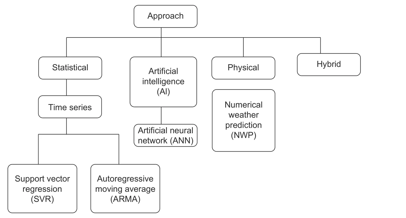
Fig.1.Forecasting techniques[9],[10].
For very short-term forecasting (minutes to few hours), on-site measured irradiance data in combination with time series models are appropriate.It can be used for PV and storage control and electricity market clearing.The models appropriate for these include Kalman filtering, autoregressive (AR), and autoregressive moving average(ARMA) models.Again, artificial neural networks (ANNs) may be applicable to derive irradiance forecasts only using the measurements[11].
On the other hand, short-term (up to 48 hours to 72 hours ahead) forecasting including information on the temporal development of clouds, which largely determine the surface solar irradiance, may be used as a basis for a short-term task like power system operation, including economic dispatch, unit commitment, etc.Moreover, the prediction, using satellite images, demonstrates good performance for up to one week ahead considered as medium-term forecasting.This is very useful for maintenance and scheduling of PV plants, conventional power plants, transformers, and transmission lines.For the sub-hour range, cloud information from ground-based sky imagers may be utilized to find irradiance measurements with much higher spatial and temporal resolution compared with the satellite-based forecasts.
However, the long-term estimation (up to months to years) forecasts based on numerical weather prediction(NWP) models typically outperform the satellite-based forecasts[12].This is very useful for long-term solar energy assessments and PV plant planning.That is why power forecasting models in the context of PV grid integration are usually based on this approach.
In the second step, the irradiance on the PV surface has to be calculated by using different possible types which are as follows:
1) For the systems with a fixed face orientation, the forecast values of GHI have to be transformed according to the particular orientation of PV modules and it needs the data of the tilt angle and orientation of the PV system as input.
2) The tracking algorithm needs to be used for one- and two-axis systems.
3) Concentrating PV systems needs data on the direct normal irradiance (DNI) which may be obtained from the GHI forecast using forecasted cloud and atmospheric parameters as input to radiative transfer calculations[13].
Finally, the prediction system of PV power output is formulated by applying a PV simulation model to the obtained irradiance from the module plane.Forecasting the solar power is broadly categorized according to the time horizon in which they generally display values.In practice, different forecasting approaches are opted depending on different scales of prediction horizons to meet the requirements of the decision[14].
3.Analysis Model
3.1.Machine Learning Algorithm
In this paper, we used a supervised learning algorithm—support vector regression (SVR) for forecasting[14],[15].Fig.2 depicts the overview of the machine learning algorithm.In our case, different weather variables are considered as the features for the regression analysis and the output (Y) is the solar irradiance.The used training set is a part of the weather and past actual solar power data, and the learning algorithm is an SVR model which obeys the structural risk minimization principle.
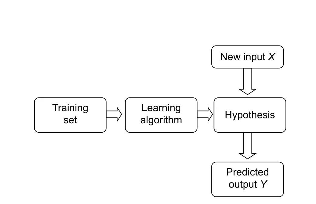
Fig.2.Machine learning flowchart.
A generalized PV power forecasting model was proposed on the basis of SVR, historical data of PV power output, and meteorological data.We analyzed this model with three distinct support-vector-machine (SVM) kernel functions including a linear kernel, a polynomial kernel, and a radial basis function (RBF) kernel[16],[17].It is observed that the RBF kernel among other kernels, using all seven dimensions to the seven weather metrics, gives a much better regression model than the other methods, as indicated by its low cross validation and forecasting errors, both of which are significantly lower than either the linear or polynomial kernels.
3.2.Weather Data Analysis
The most significant variables in the solar PV generation model are time, date, and weather[18],[19].In order to choose predictors in the PV forecasting model, the sky cover, relative humidity, dew point, temperature, wind speed, pressure, and precipitation need to be considered as weather variables.Next, the data were divided into two sections, i.e., training and testing.Comprising of eight different input parameters, a dataset of 96 values was considered for three cities.And the complete dataset for one of the cities is mentioned in Table 1.For better accuracy and learning, we have considered our data analysis for eight different regions, out of which we have demonstrated and analyzed the result for three cities including City-A (23.8103° N, 90.4125° E), City-B (22.3569° N,91.7832° E), and City-C (22.7010° N, 90.3535° E).The rest was used as test data.
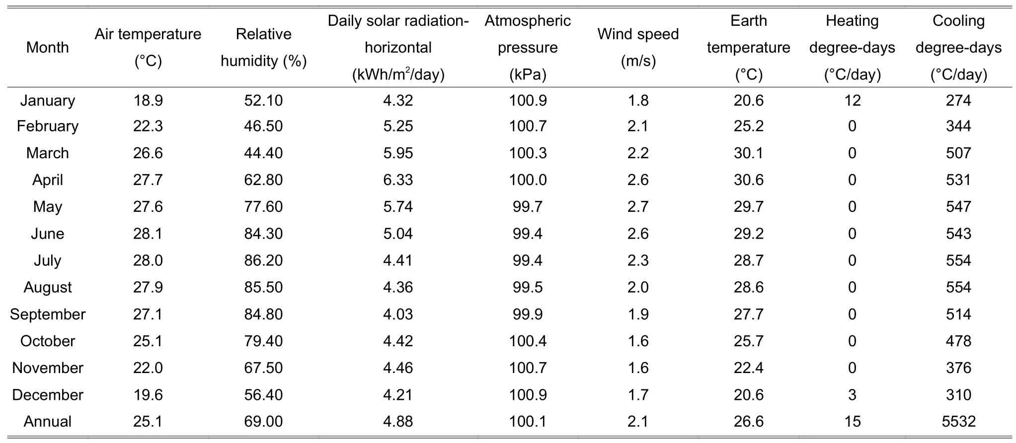
Table 1:Daily solar radiation for City-A (23.8103° N, 90.4125° E) under different weather conditions
3.3.Simulation and Analysis
The SVR classifier is trained with the weather data set where the followings were considered as features:Monthly mean values of minimum temperature, maximum temperature, sunshine duration hour, pressure, earth heating temperature, and earth cooling temperature.The solar irradiance is considered to be the output.For the learning process, 87.5% of the data were used for training the classifier and the remaining 12.5% for testing the model.
Among the kernel functions, the radial basis and polynomial functions were implemented for the SVR prediction of solar irradiation.The SVR analysis accuracy broadly relies on the model parameter clarification; it is designed to figure out which function has the highest number of deviationsεfrom the actual destination vector for flat training data.Therefore, the optimal values of the regularization factorCand the size of the error in the sensitive area inεmust be established.The optimization of these settings controls the complexity and forecasting.For this work, the values of the parameters were based on the trial and error approach and the best combination of these parameters was chosen.
From Fig.3, it is found that, for City-A, the highest predicted value occurred in March and the lowest in September.
Likewise, the same phenomena occur with slight variations for City-B and City-C, as shown from Fig.4 to Fig.8.But in Figs.7 and 8, the estimated and experimental values vary significantly for the reason that the data used for this analysis were not sufficient enough in those areas.For instance, in those areas,the cloud coverage and sun elevation angle are very important to define the solar radiation, but they cannot be incorporated in this study due to the unavailability of these data.But still the prediction exhibits reasonable output.Hence it can be mentioned that the overall prediction accuracy for each city is found to be reasonable,which validates the forecasting model.
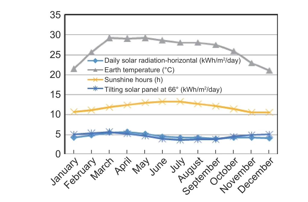
Fig.3.Actual daily solar radiation for City-A (23.8103° N, 90.4125° E) under different weather variables using geographic information system (GIS) data.
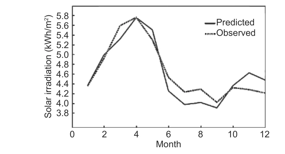
Fig.4.Predicted and observed daily solar radiation using actual and training data, respectively, to compare the model accuracy for City-A under different weather conditions.

Fig.5.Actual daily solar radiation for City-B (22.3569° N,91.7832° E) under different weather variables using GIS data.
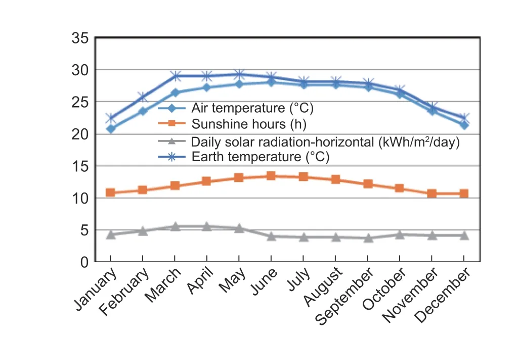
Fig.6.Actual daily solar radiation for City-C(22.7010° N, 90.3535° E) under different weather variables using GIS data.
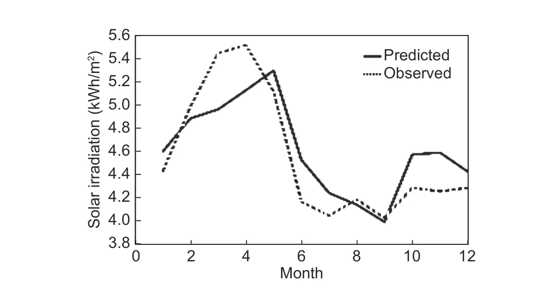
Fig.7.Predicted and observed daily solar radiation using actual and training data, respectively, to compare the model accuracy for City-B under different weather conditions.
4.Voltage Stability Analysis: Renewable lntegration
It is increasingly important for grid operators to understand how they can reliably integrate large quantities of RE into system operation.A block diagram for interfacing the PV array to the grid is given in Fig.9.It becomes important to enable these new solar power plants to provide much-needed essential reliability services (e.g.,frequency and voltage support) that can improve the reliability and resilience of the electric grid.
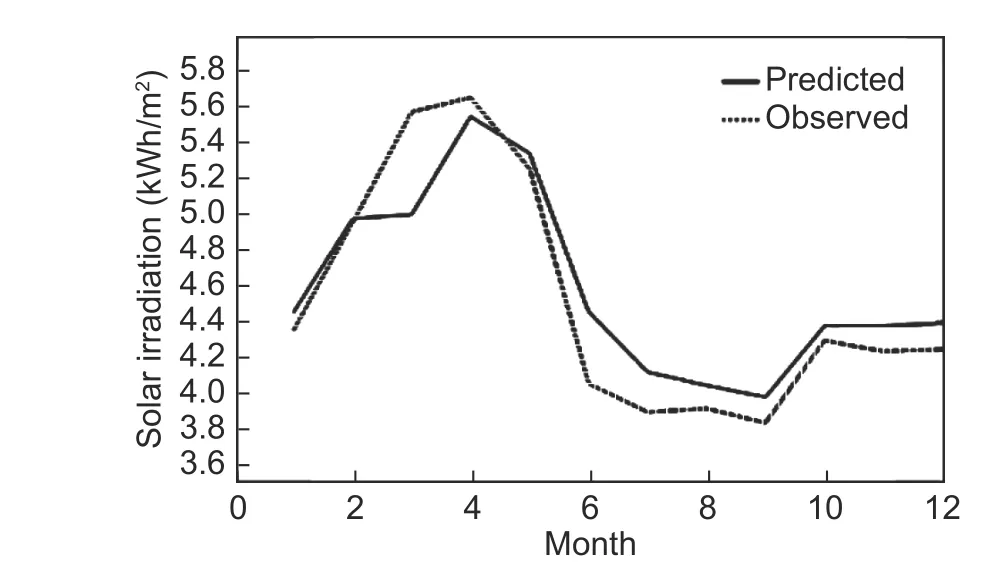
Fig.8.Predicted and observed daily solar radiation using actual and training data, respectively, to compare the model accuracy for City-C under different weather conditions.
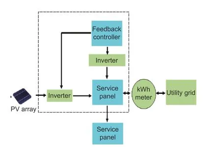
Fig.9.Block diagram for grid interface with PV array.
To investigate the voltage stability, a three-machine,seven-bus system was proposed as a platform and this was further extended by inserting a flexible AC transmission systems (FACTS) device into the system.A thyristor controlled series capacitor (TCSC) shown as Fig.10 was added to the power network to provide dynamic voltage control and dynamic power flow control for the transmission lines, relieve transmission congestion, and improve power oscillation damping(POD)[20],[21].The subsequent simulation results show that the FACTS device could significantly improve the performance of the power network during transient disturbances.
A series compensation technique involving thyristor control was provided for the rapid dynamic modulation of the given reactance.Depending on interconnections between transmission grids, this device can give strong damping torque on inter-area electromechanical oscillations.Usually TCSC is inserted with a fixed series compensation to enhance the transient stability in an effective way.The dynamic model of TCSC drawn in Fig.11 depicts the following two basic principles.
1) TCSC provides electromechanical damping torque by changing the reactance of a specific interconnecting power line.
2) TCSC effectively controls a potential sub synchronous resonance by inter-changing its impedance from capacitive to inductive for low frequencies as assumed by the line current.
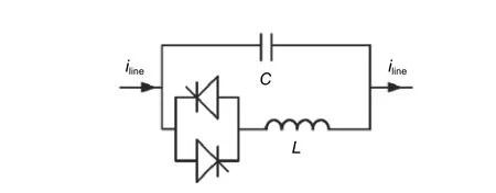
Fig.10.Structure of TCSC.
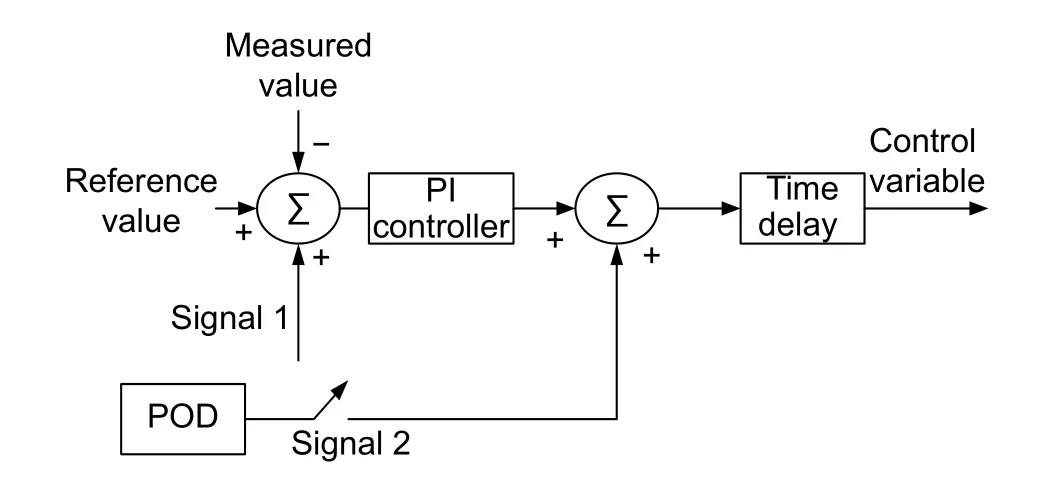
Fig.11.Dynamic model of TCSC.
4.1.Dynamic Model of TCSC
By just adding the FACTS device without control,the damping was not increased.To increase the damping (shown in Table 2) of the inter area mode,POD is used.
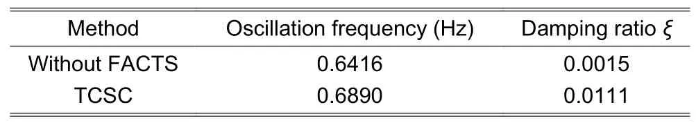
Table 2:Devices (no POD) effects on the inter-area mode
4.2.lnter-Area Mode
The power oscillation modes can be classified as: i) local modes and ii) inter-area modes[21],[22].The local modes are referred to as the rotor angle oscillation of a generator swings against the rest of the power system, and the inter-area modes are the oscillations between groups of generators from one area to another one.
4.3.Control with TCSC
After analyzing the network of Fig.12 without the FACTS device, it was observed that the damping ratio was critically low, which indicates that the system might move to instability if it keeps on running without further measures.Hence, different control methods were opted for finding a better control strategy to damp out the oscillations as well as inserting POD in a proper place was investigated and is summarized in Table 3.The filter withT1andT2was used for phase regulation (to make the input and output of the POD controller in an exact opposite phase) and KPOD was the POD gain which was determined based on the desired damping coefficient.It was found that using the control Lyapunov function (CLF) control signal worked better than other methods.Moreover, after the insertion of TCSC, the damping ratio was increased and also the gain was enhanced.Hence, the FACTS device could reduce the oscillations in the grid, which is especially a major concern issue when dealing with the stochastic behavior of renewables.From this finding, it can be further illustrated that the controllability of TCSC provides the network shown in Fig.12 much more flexibility to incorporate renewables and properly manage their intermittent nature.
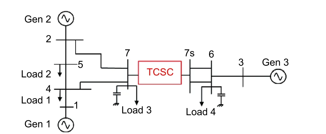
Fig.12.Layout of the analyzed network with the FACTS device.
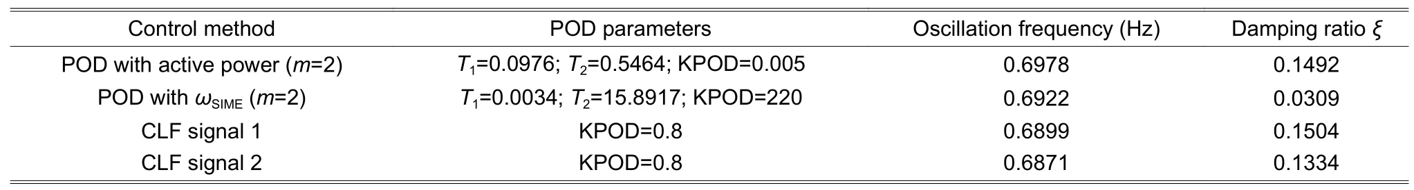
Table 3:Simulated parameters with the FACTS device
4.4.Fault Case Study
Another important issue about the renewable integration is the way that the solar generation reacts to faults or voltage excursions.At the transmission level, solar power can be controlled to keep the system in synchronization during faults of limited duration.However, current standards (Institute of Electrical and Electronics Engineers (IEEE)1547) need distribution-level solar to quickly disconnect during these events.The result is that it may be more difficult to avoid or recover from such system disturbance in a prompt way.In order to analyze the effect of different control strategies of controllable components used in multi-machine power systems (MMPSs), the single machine equivalent method (SIME) model is used.
The SIME method assesses the post-fault configuration of MMPS by replacing the trajectories of MMPS with the trajectory of a one-machine infinite-bus system with a following form:
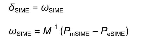
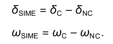
whereMis the inertia constant;PmSIMEandPeSIMEare the equivalent mechanical input power and the equivalent electrical output power, respectively.After subjecting the power system with disturbance, which supposedly leads the system to instability, and using time domain program, the mode of instability is identified where machines are separated into two groups, i.e.critical machines (subscript C) and non-critical machines(subscript NC).The SIME parameters for these critical machines are as follows:
In our system, a single line to ground fault (L-G-F) is applied just to figure out the system response when the FACTS device is already installed.Observability is investigated for the FACTS device by using both the local signal and the remote output signal (ωSIME) from the system.The local signal is the active power flowing in between bus 3 and bus 6 (P3-6).
From the simulation of large disturbance shown in Fig.13, it is found that all POD is designed with the remote signalωSIMEand the CLF method provides the best response damping of the oscillations.Hence, TCSC including POD can improve both the voltage and transient stability of the power system by enhancing the voltage profile as well as reactive power support by suppressing the oscillation modes.
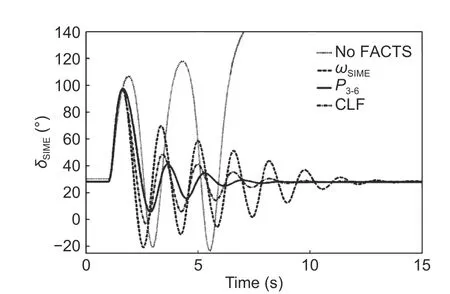
Fig.13.Fault for the large disturbance in the given network (major disturbance bus 7).
5.Conclusion
All electric grids are different and the optimal solutions for addressing integration depend on the challenges associated with the variability and uncertainty of RE generation.It is found that the least-cost options available to individual grids mostly depend on the overall flexibility of the grid because of the generation mix (including the RE penetration), regulatory structure, presence or absence of markets, operational practices, and institutional structures[23].Moreover, alternative methods of managing the resources may be possible and could result in more enhanced efficiency with higher penetrations of renewables.Finally, better understanding of the forecasting of solar generation sources with higher accuracy and the issues related with the integration of RE in the grid for assessing flexibility could be useful to identify and evaluate more practical and efficient solutions.
Disclosures
The authors declare no conflicts of interest.
杂志排行

Journal of Electronic Science and Technology的其它文章
- Smart Meter Development for Cloud-Based Home Electricity Monitor System
- Comparative Study of 10-MW High-Temperature Superconductor Wind Generator with Overlapped Field Coil Arrangement
- Characteristic Length of Metallic Nanorods under Physical Vapor Deposition
- Computational lntelligence Prediction Model lntegrating Empirical Mode Decomposition,Principal Component Analysis, and Weighted k-Nearest Neighbor
- Data Bucket-Based Fragment Management for Solid State Drive Storage System
- ECC-Based RFlD Authentication Protocol