Developing a process-based and remote sensing driven crop yield model for maize (PRYM–Maize) and its validation over the Northeast China Plain

ZHANG Sha ,BAi Yun ,ZHANG Jia-hua , ,Shahzad Ali

1 School of Automation,Qingdao University,Qingdao 266071,P.R.China

2 College of Computer Science and Technology,Qingdao University,Qingdao 266071,P.R.China

3 Aerospace Information Research Institute,Chinese Academy of Sciences,Beijing 100094,P.R.China

4 University of Chinese Academy of Sciences,Beijing 100049,P.R.China

Abstract Spatial dynamics of crop yield provide useful information for improving the production. High sensitivity of crop growth models to uncertainties in input factors and parameters and relatively coarse parameterizations in conventional remote sensing(RS) approaches limited their applications over broad regions. In this study,a process-based and remote sensing driven crop yield model for maize (PRYM–Maize) was developed to estimate regional maize yield,and it was implemented using eight data-model coupling strategies (DMCSs) over the Northeast China Plain (NECP). Simulations under eight DMCSs were validated against the prefecture-level statistics (2010–2012) reported by National Bureau of Statistics of China,and inter-compared. The 3-year averaged result could give more robust estimate than the yearly simulation for maize yield over space. A 3-year averaged validation showed that prefecture-level estimates by PRYM–Maize under DMCS8,which coupled with the development stage (DVS)-based grain-filling algorithm and RS phenology information and leaf area index (LAI),had higher correlation (R,0.61) and smaller root mean standard error (RMSE,1.33 t ha–1) with the statistics than did PRYM–Maize under other DMCSs. The result also demonstrated that DVS-based grain-filling algorithm worked better for maize yield than did the harvest index (HI)-based method,and both RS phenology information and LAI worked for improving regional maize yield estimate. These results demonstrate that the developed PRYM–Maize under DMCS8 gives reasonable estimates for maize yield and provides scientific basis facilitating the understanding the spatial variations of maize yield over the NECP.

Keywords:process-based and remote sensing model,maize yield simulation,development stage,grain filling,harvest index

1.introduction

The increasing food demand has become an urgent issue over the globe due to the rapid increase of global population (Sonet al.2013). However,crop land expansion has induced serious environmental problems in the past decades (Lobellet al.2009). Therefore,exploring the crop yield potential and finding ways to increase the crop yield were the global priority. Achieving the goal requires a comprehensive understanding of crop yield over time and space (Huanget al.2018). However,accurately mapping crop yield on a regional,national or global scale remains challenging limited by the models’ applicability and region data availability (Yaoet al.2007,2011; Zhanget al.2015;Wanget al.2020).

The crop growth model (CGM) is a reliable tool for crop yield estimates. Multiple CGMs have been exercised to predict crop yield over the globe due to their high efficiencies (Lobellet al.2009; van Ittersumet al.2013).And they provide useful information for site-scale analyses(Zhanget al.2013; Sunet al.2015). Series of CGMs have been developed,e.g.,Hybrid–Maize (Yanget al.2004),APSIM (Mccownet al.1996),WOFOST (Supitet al.1994),and DSSAT-CERES (Bassoet al.2016). The calibrated CGM reliably estimates crop yield within a given region (Chenet al.2010; Wanget al.2014; Amarasinghaet al.2015; Inneset al.2015). The accurate simulation of a CGM relies on reliable meteorological data (Wartet al.2013) and field management information (Zhanget al.2013; Amarasinghaet al.2015),and the model outputs crop yield of the cropland where a meteorological site nearby. Therefore,there are two problems when applying CGMs over broad regions. One was caused by the sparse distribution of weather stations on a national or global scale,Wartet al.(2013) proposed a protocol to resolve this issue. However,their method could cover just approximately 40–50% of the crop lands being investigated over a country. The limited detailed field management information over broad regions caused another question,i.e.,the field managements of different fields within a domain under investigation were usually assumed to be homogenous when using CGMs. Actually,the crop yield and agricultural landscape have great heterogeneity in time and space (Lobell 2013; Zhaoet al.2016).

The use of remote sensing (RS) approaches may be an alternative way to address the two issues mentioned above (Huanget al.2015; Gilardelliet al.2019). RSbased approaches are more applicable on a regional scale,because these methods are forced by remotely sensed crop growth information which is free from the effect of the uncertainties in meteorological data. Previous studies have found improvement in crop yield simulations facilitated by RS (Curnelet al.2011; de Witet al.2012; Balkovičet al.2013; Huanget al.2015). Field or pixel-level crop growth information provided by RS could also reflect the on-farm managements. Therefore,the remotely sensed methods provide spatial dynamics of field or pixel-level crop yield.RS data have long been utilized in land process models to simulate ecosystem productivities,thus,it is potentially useful for crop yield estimates. Wanget al.(2011) modified the process-based model,Boreal Ecosystem Productivity Simulator (BEPS),and successfully used it to simulate the yield of winter wheat over North China Plain. Yaoet al.(2015) used the same method to estimate the maize yield over the Northeast China. Light use efficiency (LUE) models and empirical approaches were more favored by a majority of recent works on RS-based mapping and spatial analyses of crop yield (Lobell 2013; Lobellet al.2013,2015; Zhaoet al.2016; Wanget al.2019),as these methods were simply formulated and could also give reasonable outputs within specific domains.

Conventional RS-based models were initially designed for modeling vegetation productivity rather than crop yield.Most RS-based models used ‘biomass×harvest index (HI)’(HI-based method) to calculate the dry matter of grains(Lobell 2013; Lobellet al.2013,2015; Zhaoet al.2016).In addition to the HI-based method,CGMs generally provide the calculation of daily grain-filling rate based on development stage (DVS) of crops (DVS-based method) to simulate crop yield (Supitet al.1994; Mccownet al.1996;Yanget al.2004; Liet al.2009; Moet al.2012; Osborneet al.2015; Bassoet al.2016; Penget al.2018). Only few previous studies used DVS-based method in RS-based models and process models to simulate crop yield. Huanget al.(2018) proposed to use normalized accumulated gross primary productivity (GPP) in a process model to estimate the daily grain-filling rate of rice,and this method successfully simulated the rice yield across six site-years in Korean peninsula. The DVS-based methods seem more reasonable,and they have stronger theoretical bases than generally used HI-based methods when calculating crop yield. Because the HI parameter,which was usually set as a constant for a specific crop in a specific region,may vary over time and space (Sinclair 1998; Juet al.2010).However,the HI-based method could outperform the DVSbased method within specific domains (Jinet al.2016,2017).Therefore,maybe both HI-and DVS-based methods are useful for calculating crop yield. But it is still unclear that which method works better with RS-based approaches over a specific region.

The major objectives of the study are:(i) to develop a process-based and remote sensing driven crop yield model for maize (PRYM–Maize) to simulate the regional yield of maize over the Northeast China Plain (NECP),apply it over the NECP under eight data-model coupling strategies(DMCSs),and validate and inter-compare the maize yield simulated using the eight DMCSs on a prefecture-level;(ii) to explore whether the DVS-or HI-based methods perform better when simulating maize yield over the NECP;and (iii) to investigate the role of RS information in regional maize yield estimation.

2.Materials and methods

2.1.Study area

The developed PRYM–Maize will be applied to estimate the regional yield of spring maize over the NECP from 2010 to 2012. The study region covers three provinces(Heilongjiang,Jilin and Liaoning) in Northeast China(0.72 million ha,38.72–51.00°N,118.84–134.78°E). It is approximated to produce 34% of the total production of maize in China (Liu 2013; Bai 2019). The study region has a humid/semi-humid monsoon climate with annual averaged temperature ranging between–4.2 and 10.9°C and precipitation ranging between 400 and 1 100 mm over space. Approximately 80% of the annual precipitation falls during the 5 mon between May and September,when the average temperature is also greater than that of the left months. The 5 mon also cover the majority of the growing season of spring maize.

2.2.Development of PRYM–Maize

We will develop the PRYM–Maize Model,which incorporates both DVS-and HI-based algorithms to partition the dry matter of grain from the total photosynthetic product of maize,in this study.

Configuration of PRYM–MaizePRYM–Maize runs on a daily step. It consists of two sub-modules (Fig.1-A),a“water balance module” and a “photosynthesis module”.The water balance module follows the “Remote Sensing and Water Balance-based Penman-Monteith Model version 2”(RS-WBPM2) (Baiet al.2018),which was modified from Baiet al.(2017),to simulate water stress. The photosynthesis module consists of a canopy-scale photosynthesis module and a grain-filling algorithm (Fig.1-B). The photosynthesis module uses a two-leaf canopy model along with remotely sensed LAI to scale leaf-level photosynthesis to canopy scale. Remotely sensed phenology information (emerging and maturity dates) was introduced into the grain-filling algorithm to estimate yield from GPP (Fig.1-B). The water balance module was according to Baiet al.(2018). The details of the photosynthesis module will be presented in following contents of this section.

leaf-level photosynthesis modelThe simple intercellular transport (ICT) Model (Berryand Farquhar 1978; Collatzet al.1992) is adopted to simulate the leaf-scale photosynthesis of maize. It has been incorporated into multiple terrestrial land process models to simulate the photosynthesis of C4plants and evidenced to be useful (Ryuet al.2011; Moet al.2012; Jiangand Ryu 2016). The equations for leaf-level photosynthesis are presented as:

whereAnis the net photosynthesis rate (µmol m–2s–1);Av,AeandAsare Rubisco,potential electron transport and export limited photosynthesis rates,respectively (µmol m–2s–1);Rddenotes the dark respiration (μmol m–2s–1),andRd=0.015Vm;Vmdenotes the maximum carboxylation rate(µmol m–2s–1);εdenotes the intrinsic quantum efficiency;Qdenotes the incident photosynthetically active radiation(PAR) on the leaf surface (µmol m–2s–1);cidenotes the intercellular partial pressure of CO2(Pa); andPatmdenotes the atmosphere pressure (Pa).

Vmwas fixed in previous versions of ICT model (Collatzet al.1992). It is calculated as a function of temperature(T) and nitrogen (N) supply in this study as that in C3photosynthesis models (Bonan 1995; Chenet al.1999; Liuet al.1999),such that:

whereVm25denotes the maximum carboxylation rate at the temperature of 25°C,it is set to 60 µmol m–2s–1for maize (Caemmerer 2000; Kimet al.2007);fT(T) represents the restrictive function of temperature;fN(N) denotes the restrictive function of nitrogen supply,which varies between 0 and 1,however,spatial information for field management or the nitrogen supply is not available,fN(N) is fixed over the NECP,0.65 is used;Rgasdenotes the mole constant of gas,8.3143 J mol–1K–1.

For potential electron transport limited photosynthesis rateε,ICT model usesε=0.067 mol mol–1for C4plants(Collatzet al.1992). In this study,εis simply assumed to be limited byfN(N) as the electron transport rate correlates well withVm(Caemmerer 2000; Medlynet al.2002),such that:

whereεmdenotes the maximum value forε,and 0.067 mol mol–1is used.

Ascould not be solved by eq.(4) alone since the value ofciis not easily obtained on a regional scale,eqs.(1)and (4) are combined with theAncalculation based on fluid physics (Leuning 1990; Chenet al.1999; Liuet al.1999) to avoidci.

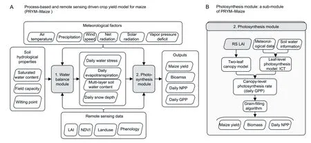
Fig.1 Flow chart of a process-based and remote sensing driven crop yield model for maize (PRYM–Maize) (A) and its photosynthesis module (B). The remotely sensed crop growth information inputs to the photosynthesis module were highlighted with dark grey background and thick border. NPP,net primary productivity; GPP,gross primary productivity; LAI,leaf area index; NDVI,normalized difference vegetation index; RS,remote sensing; ICT,intercellular transport.

wherecadenotes the partial pressure of CO2in the atmosphere,it is fixed to 39 Pa;g(gst) denotes the stomatal conductance measured in µmol m–2s–1Pa–1;gstdenotes the stomatal conductance measured in m s–1. Combining eqs.(1),(4) and (8),we get a form ofAsin terms ofgrather thanci:

Canopy-level photosynthesis model on a daily scaleA two-leaf canopy structure model based on the radiative transfer theory (Norman 1982; Chenet al.1999; Liuet al.1999) is used to scale leaf scale photosynthesis rate to a canopy scale. The two-leaf model showed good reliability in simulating canopy scale photosynthesis rate (Chenet al.1999; Ryuet al.2011). And a two-leaf photosynthesis model on a canopy and daily scale is shown as follows:

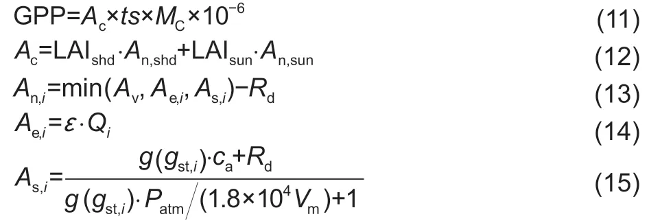
where GPP denotes the daily gross primary productivity on a canopy scale (g C m–2d–1),Acdenotes the net photosynthesis rate on a canopy scale during the daytime (µmol m–2s–1);tsdenotes the temporal scale of the model,ts=Hrday×3 600 s,Hrday,the possible sunshine duration in hours (from sunrise to sunset),and is calculated according to Duffieand Beckman(2013);MC,the mole mass of carbon (12 g mol–1); shd and sun,the shaded and sunlight leaves,respectively,andi,shd or sun; LAI,leaf area index; LAIshdand LAIsun,the leaf area index of shaded and sunlight leaves,respectively; andAn,shdandAn,sun,theAnvalue of shaded and sunlight leaves,respectively.

LAIsunand LAIshdare partitioned from the total leaf area index on a canopy scale,we refer to Chenet al.(1999),Liuet al.(1999) and Norman (1982) for the calculations(Appendix A). Instead of being simulated using the crop growth model,the canopy scale LAI used for calculating LAIsunand LAIshdin PRYM–Maize is retrieved from the remote sensing images.

On a daily basis,gst,iis calculated using the canopy conductance model RST-Gcdeveloped and optimized by Baiet al.(2018):

wheref1(VPD),f2(Qi),f3(T),andf4(swc) are restrictive functions of vapor pressure deficit (VPD),photosynthetically active radiation (PAR,Q),air temperature (T),and soil water content (swc).QsunandQshdare two critical variables in canopy photosynthesis simulations with a two-leaf canopy structure. In terms of eqs.(1)–(4) and (10),calculations ofAn,shdandAn,sunrequireQandgston shaded leaves (Qshdandgst,shd) and sunlight leaves (Qsunandgst,sun),and calculations ofgst,shdandgst,sunare also based onQsunandQshd(Baiet al.2018). The calculations ofQsunandQshdare referred to Norman (1982),Chenet al.(1999) and Liuet al.(1999)(Appendix B).

Grain-filling algorithmsTwo types of methods,DVS-and HI-based algorithms,were used to calculate grain-filling of crops in PRYM–Maize.

(1) DVS-based grain-filling algorithm

In the DVS-based grain-filling algorithm of PRYM–Maize,maize yield is estimated using the following formulas:

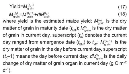
We refer to the ‘Vegetation Atmosphere Interface Processes (VIP) Model’ for calculating the daily change of dry matter accumulation for an organ ‘x’ of maize (Moet al.2012).

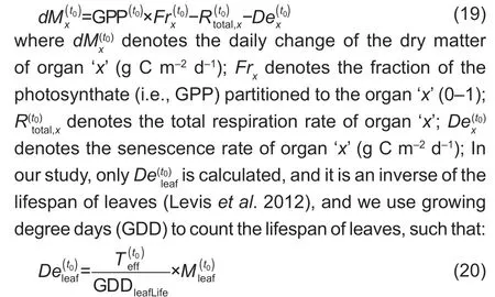
The dry matter allocation method adopted by Osborneet al.(2015) is used to the fraction of daily GPP partitioned to organ ‘x’ (Frx) in this study. This method calculatesFrxas a function of the DVS that is determined by accumulated effective temperature.The method to calculate theFrxof leaf,stem and root is presented as following:

andFrgrainis the residual of theFrxvalue of the three organs above:

whereaxandbxwere empirical coefficients,which controlled the shape of the curve ofFrx; DVS denotes the development stage of the crop (0–2),and DVS=1 indicates the flowering when the accumulation of grains starts; DVS=2 indicates the maturity stage. We did not use the coefficient values adopted by the Joint UK Land Environment Simulator(JULES) Model (Osborneet al.2015),but adjusted theaxandbxvalues based on the observations of Haoet al.(2016)to optimize the estimate ofFrgrain(Table 1). When conducting the adjusting process,theaxparameters were maintained unchanged,and a scale factor,which varied from 0.10 to 2.00 with a step of 0.05,was used to scale thebxparameters.The value of the scale factor was determined when it minimized the RMSE value between theFrgrainvalues,calculated by eq.(22),and the observations. The scale factor turned out to be 0.80. The values ofaxand adjustedbxare shown in Table 1. The adjusted parameters yieldedFrgrainthat agreed well with the observations (Appendix C)but departed significantly from the values before adjusting(Appendix C).

The DVS is calculated as a function of the accumulated daily effective air temperature (or growing degree days)(Supitet al.1994; Osborneet al.2015; Haoet al.2016):

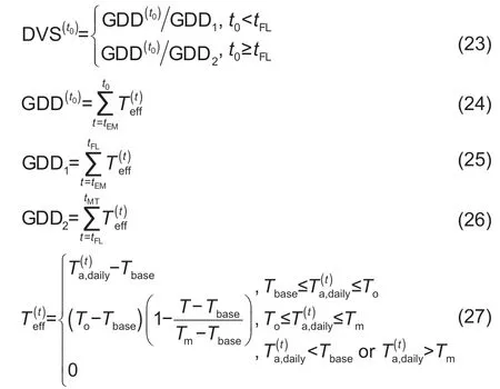
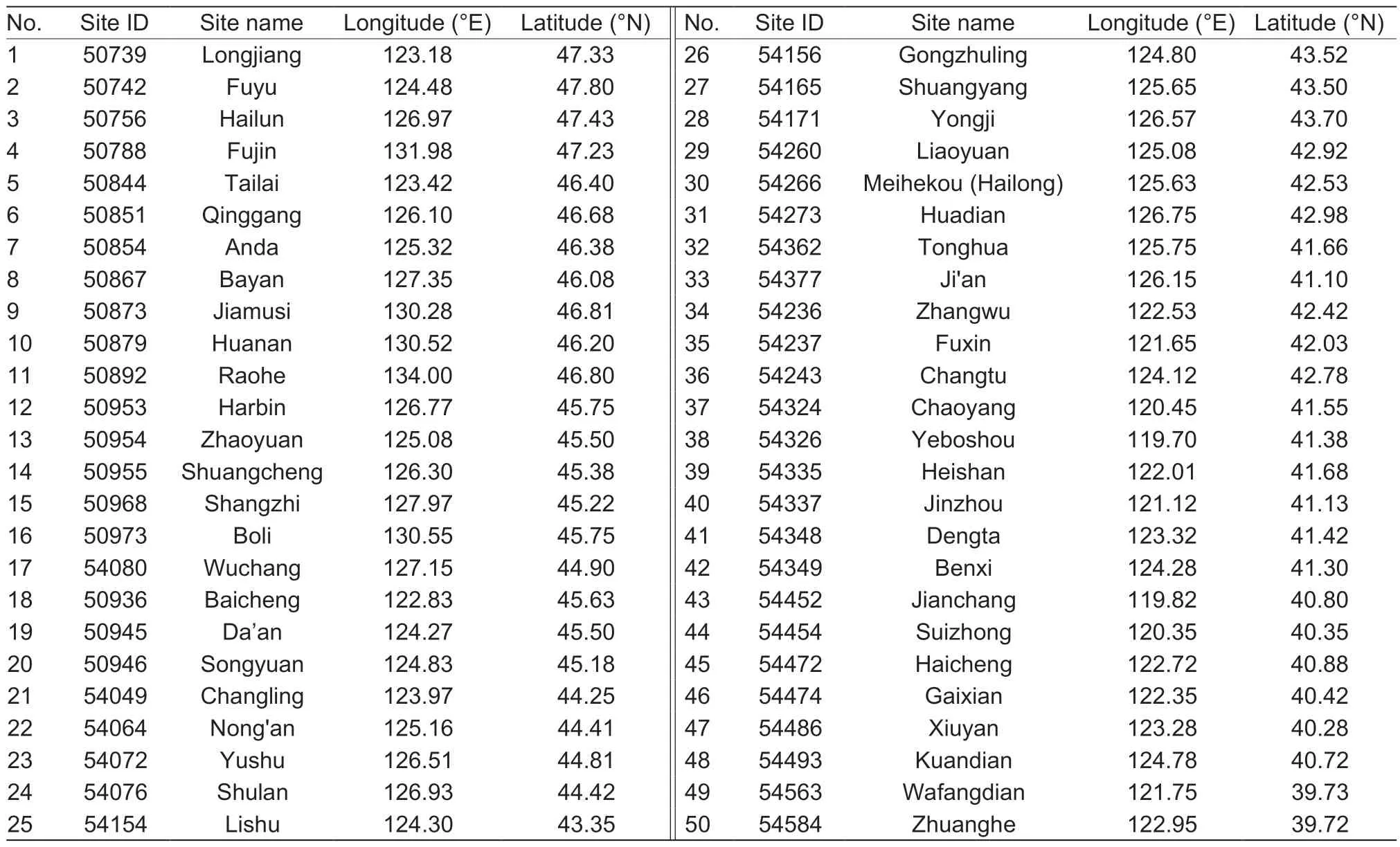
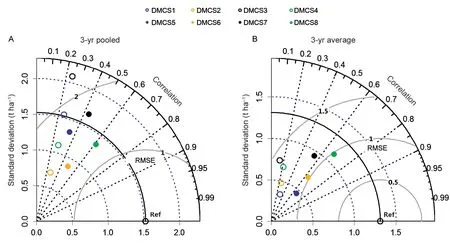
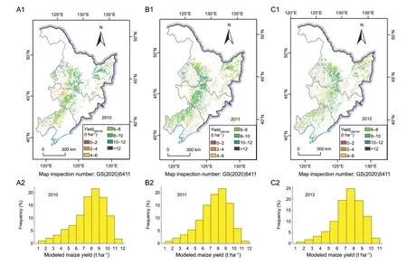
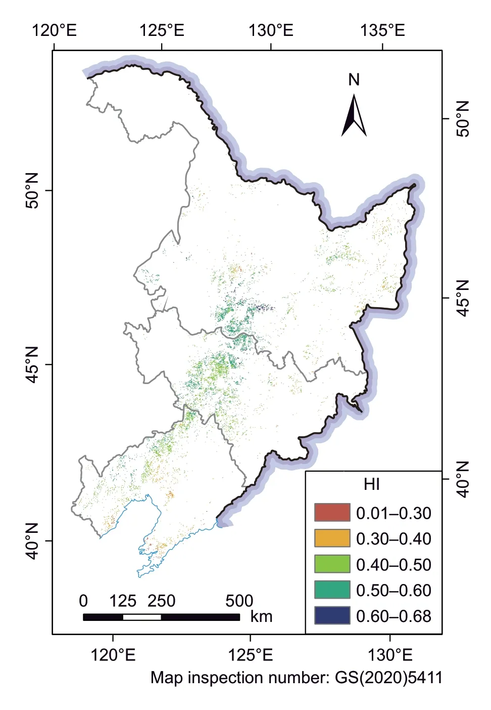
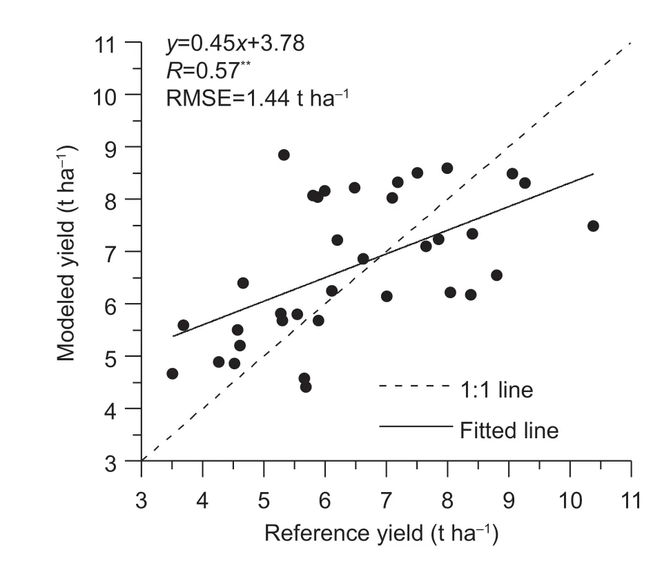
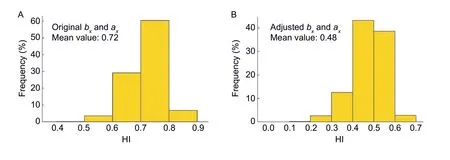
where GDD1and GDD2are the accumulated daily effective air temperatures (or growing degree days) required for flowering and maturity (°C d);Teffdenotes the effective air temperature;tEM,tFLandtMTdenote the dates of emerging,flowering and maturity,respectively;denotes the daily temperature (°C);Tbase,ToandTmare the base,optimum and maximum temperatures for crop developments,respectively,Tbase

tFLwas a necessary input (eq.(23)). A linear relationship betweenJFLandJMTis feasible to estimatetFLwhen timeseries RS-retrieved VI is available,whereJFL=tFL–tEMandJMT=tMT–tEM

wherek´´ andb´´ are empirical coefficients.

A calibration for the linear relations betweenJFLandJMT(eq.(28)) is shown in Appendix C. Observed data of the emergency,flowering and maturing dates were required.These data were retrieved from published works (Ouyang 2010; Zhanget al.2010,2014; Liuet al.2012) and field trails. The coefficientsk´´ andb´´ in eq.(28) turn out to be 0.418 and 6.83 (Appendix C),respectively. The number ofdays for maize developing from emerging to maturity (JMT)is determined by TIMESAT-retrieved SoS and EoS,i.e.,JMT=EoS–SoS,the SoS and EoS mean start and end of growing season,respectively.

Table 1 The original and adjusted values of coefficients ax and bx which are related with maize dry matter partitioning simulation(eqs.(21) and (22))

(2) HI-based algorithm

The HI-based method was generally incorporated by conventional RS-based models to calculate the yield of crop(Taoet al.2005; Wanget al.2011; Lobell 2013),and was presented as the follow:

whereMgrain,the dry matter of grain,which is equivalent to the crop yield; the HI of maize was fixed to 0.45 over the NECP (Lv 2016);dM(t0),the dry matter change of the whole maize plant at dayt0;,the total respiration rate of the whole plant.

Daily respirationRespiration is non-ignorable in the carbon budgets processes between ecosystems and the atmosphere,which was included in PRYM–Maize.It is feasible to estimate respiration as a fixed fraction of photosynthesis product (i.e.,GPP). However,the proportion of respiration to GPP varies over time and space,as it tightly correlates with temperature (Amthor 1984). In this study,we calculate respiration in terms of daily temperature. The total respiration (Rtotal) consists of maintenance respiration(Rm) and growth respiration (Rg),referring to Chenet al.(1999) and Liuet al.(1999):

whereRtotal,RgandRmare daily total,growth and maintenance respiration rates (g C m–2d–1);Q10denotes the temperature sensitivity parameter of respiration reflecting the increments of respiration rate with an increase of temperature by 10°C,a value of 2 is used for all cases (Yanget al.2004);rgdenotes the growth respiration coefficient (0.25) (Amthor 1984);rmdenotes the maintenance respiration coefficient. For the DVS-based methods,daily respiration rates of different organs were calculated;rmdiffers among different organs of the maize plant,the values ofrmfor grain,leaf,stem,and root are shown in Table 2. For the HI-based method,onlyRmof the whole plant is required,rmis the maintenance coefficient for a whole plant,the average ofrmvalues presented in Table 2 are used to calculate theRmof the whole maize plant along with eq.(33).

2.3.Model forcing strategies

In this study,the model will run under eight DMCSs as shown in Table 3. DMCS1–4 are with HI-based grain-filling algorithm,and DMCS5–8 are with DVS-based grain-filling algorithm.In DMCS1–4,the phenology and LAI data couplings are different,so are in DMCS5–8. By comparing the yields estimated from PRYM–Maize under the eight DMCSs,we will answer the three questions:(i) does a more complicatedly formulated DVS-based grain-filling algorithm work better than the conventional HI-based method over the study region? (ii) will the RS information enhance the precision of the estimate of maize yield? (iii) do all or only one types of the RS inputs facilitate the simulation of the model?

2.4.Data and data processing

Remote sensing retrieved crop phenologyRemotely sensed normalized difference vegetation index (NDVI)retrieved from the 1-km and 16-day MOD13A2 and MCD13A2 products were used to derive the crop phenology information. The retrieved data were pre-processed in terms of the following procedures before use for avoiding unreliable data and data noise:

Quality control:values of pixels with snow or cloud cover in the retrieved data were replaced by linearly interpolating the nearest available pixels in time.

Time-series filter:TIMESAT3.3 was used to filter the retrieved VI data.

Temporal interpolation:NDVI data were linearly interpolated to the daily.

The emergence (EM) and maturity (MT) dates correspond to the start and end of season (SoS and EoS) defined in TIMESAT. Key parameters required in TIMESAT were set as the follows:

Fitting method:Double logistic

Start of season method:Seasonal amplitude

Season start/end value:0.1/0.4

The retrieved EM and MT were validated using the observed phenology dates at the agro-meteorological sites.

Observed site-scale EM and MT dates of spring maize in 2010 over NECP were used to validate TIMESAT derived maize phenology. These data were retrieved from the observations of agro-meteorological monitoring sites(Table 4) which were available on the website of National Meteorological Information Center (http://data.cma.cn/). But it is inappropriate to validate the remotely sensed phenology information by comparing the phenology data of the pixel where an agro-meteorological site stood against the site observation,because the agro-meteorological sites are usually located in the pixels on the edge of cities or villages,bringing big errors for the extracted phenology information from the remotely sensed phenology information. Therefore,for validating the remotely sensed phenology information,we used the site-observed phenology to compare against the mean value of pixels covered by the circle with a 5-km radius,which took an agro-meteorological site as the center. The TMESAT-retrieved phenology information was compared against the site-observed data (Appendix C). The observed EoS (DoY) ranged from 130 to 155 (an average of 144)with a mid-correlation (0.54) with the TIMESAT-retrieved data,and observed SoS (DoY) ranged from 265 to 275(an average of 268) with a correlation (R) of 0.70 with the TIMESAT-retrieved data. These results indicate that the SoS and EoS of spring maize over the NECP varied over space can reasonably capture the spatial trend of them.

Table 2 Values of the maintenance respiration coefficient for the grain,leaf,stem,and root of maize1)

Remotely sensed lAiLAI of maize was not directly retrieved from the MODIS product as crop LAI was reported to be significantly underestimated by the MODIS product(Yanget al.2006). In this study,maize LAI was calculated using the empirical equations,calibrated by Baiet al.(2018),in terms of enhanced vegetation index (EVI) retrieved from MOD13A2 and MYD13A2. This method was calibrated with flux-site observed maize LAI in the US,Europe and China.The method used to calculate LAI from EVI is shown as the follow:

Remotely sensed maize cultivation areasThe remotely sensed maize cultivation areas in 2010 were the results of Zhanget al.(2019). The method of Zhanget al.(2019)was improved from Zhanget al.(2014). MODIS EVI data(16 d,250 m) and observed phenology information at agro-meteorological sites were employed,and the detailed mapping procedure was found in the study of Zhanget al.(2019). The obtained maize cultivation areas were with 250 m resolution. The accuracy of maize cultivation areas was validated using official statistical data. TheR2(RMSE)of extracted maize areasvs.statistical areas were 0.86(110.97 km2) and 0.82 (25.47 km2) at prefecture and county levels,respectively. Suppose that the maize planted areas would not change a lot in following two consecutive years,the maize planted areas in 2010 were used to mask the simulated results in 2011 and 2012.

Meteorological dataGridded daily meteorological data retrieved from the European Centre for Medium-Range Weather Forecasts (ECMWF) interim reanalysis (ERAInterim) dataset and multi-site data of China Meteorological Administration (CMA) were used to drive PRYM–Maize.Surface net radiation (Rn),vapor pressure deficit (VPD) and air temperature (T) were directly retrieved from the ERA-Interim dataset. Precipitation (P) and global solar radiation(Rg) were retrieved from CMA multi-site data. Site-scale CMA data were spatially interpolated to raster dataset using inverse distance weighted method.DailyRgdata were calculated from the interpolated site-observed daily temporal range (TR) and daily sun hours (HrS) of rather than directly retrieving from the site-scale observations,because sites observedRgis too sparse to be interpolated.We refer to Chenet al.(2004) for calculating dailyRg,such that:

Table 3 Eight data-model coupling strategies (DMCS)

Table 4 Information of agro-meteorological sites used in this study

wherea,b,c,anddare empirical coefficients. The averaged values for the four coefficients over China were used,which area=0.04,b=0.48,c=0.83,andd=0.11. ERA-Interim provides gridded global meteorological variables from 1981 to the current in multiple temporal and spatial resolution.Variables from ERA were in 12-h temporal and 0.125-arcdegree spatial resolution. The daily value of one variable is the average of two 12-h values in 1 d.

3.Results

3.1.Maize yield estimates with eight DMCSs

Comparisons of pooled and 3-yr averaged validationsOn-farm yield of spring maize from 2010 to 2012 over the NECP were simulated using PRYM–Maize under eight DMCSs as detailed in Fig.2. The simulations were validated against the statistics reported by the National Bureau of Statistics of China,on a prefecture level. Pooled and 3-yr averaged validations are conducted respectively (Fig.2). It can be seen that the 3-yr averaged validation for each of PRYM–Maize under eight DMCSs (Fig.2-B) shows a better agreement with the reference values than do the pooled validation (Fig.2-A),implying that averaged simulations may give more robust estimate for maize yield. In the following analysis,we use the 3-yr averaged validation result.

Comparisons of DVS-and Hi-based simulationsIn the eight DMCSs,there are four pairs of HI-and DVSbased simulations (HI-M0R and DVS-M0R (i.e.,DMCS1 and DMCS5),HI-M1RPheno and DVS-M1RPheno (DMCS2 and DMCS6),HI-M1RLAI and DVS-M1RLAI (DMCS3 and DMCS7),and HI-M2R and DVS-M2R (DMCS4 and DMCS8)),using same driven inputs. In each pair,the DVS-simulation has a higher (lower)R(RMSE) than the corresponding HI-simulation (Fig.2-B). The largestRdifference between DVS-and HI-simulation in each pair appeared in the fourth pair,DVS-M2R and HI-M2R,reached approximately 0.35. The four dots representing the results of DVS-based grain-filling algorithm have smaller distances to the reference point than the four circles that represent the results of corresponding HI-based method. This means the DVS-based grain-filling algorithm performs better than HI-based grain-filling algorithm for maize yield simulation using the developed PRYM–Maize in NECP. The developed PRYM–Maize can be used to depict detailed dry matter allocation process of maize growth at a regional scale.

Fig.2 Taylor diagrams for validating simulated prefecture-level maize yield,with data-modeling strategies,against the reference data. A,pooled validation for all prefecture-level predictions from 2010 to 2012. B,the validation for 3-yr (2010–2012) averaged prefecture-level predictions. The point ‘Ref’ represent the reference location for all model predictions. A smaller distance of the colored point to the reference point corresponds to a higher precision of model prediction. RMSE,root mean standard error.DMCS1–8,eight data-mode coupling strategies.

Comparisons of simulations using different phenology and lAi coupling strategiesDifferent phenology and LAI coupling strategies are used to drive PRYM–Maize in this study. Among the four DVS-based simulations(DMCS5–8),DMCS5 (blue dot) and DMCS8 (green dot)have the largest and smallest distances to the reference point,respectively,in the 3-yr averaged validation. This implies that both RS-phenology information and RS-LAI provide useful information to improve the accuracy of maize yield estimate. The distances between simulations and reference point are DMSC5>DMSC6>DMSC7>DMSC8,which means the DMSC8 simulation is the closest to the reference value among the four DVS-based simulations.This implies using remote sensing phenology improves the maize yield simulation more than using fixed phenology parameters,and using remote sensing LAI could improve the maize yield simulation more than using remote sensing phenology information. The reason for the former is that the phenology information of maize,such as emergence,flowering and maturity,are various rather than a constant in space. The explanation for the latter is that LAI plays more important role than phenology information in PRYM–Maize for simulating maize yield. Because the remote sensing LAI derived from remote sensing vegetation index (EVI in this study) could reflect the real condition of maize growth,including not only phenology features (e.g.,SoS,EoS,length of season (LOS)) but also peak value of LAI. The peak LAI during growing season is essential to the maize biomass therefore yield (Bai 2019; Houet al.2020). Coupling both remote sensing phenology and remote sensing LAI provides the most useful information than only using either of the two for estimating maize yield. Thus,it’s easy to understand that PRYM–Maize under DMSC8 get the highest simulation accuracy,withR=0.68 and RMSE=1.06 t ha–1.

3.2.Spatial distribution of simulated maize yield

From Section 3.1,simulation using PRYM–Maize under DMCS8 is chosen as the best among eight DMCSs. Here,only the spatial and frequency distributions from PRYM–Maize under DMCS8 are shown (Fig.3). In the 3 years,the maize yield in NECP mainly distributed in 6–10 t ha–1,and pixels with these values were mainly in the middle part of NECP. The high-yielding (higher than 10 t ha–1) pixels occupied less than 15% of the total maize pixels in each year with,2010 having the most high-yielding pixels. The high-yielding pixels were sporadically mixed with the pixels with values of 6–10 t ha–1. In general,PRYM–Maize has the ability of capturing the main distribution features of maize yields in NECP.

Fig.3 The maps (A1,B1 and C1) and frequency distributions (A2,B2 and C2) of modeled maize yield over the Northeast China Plain (NECP) by the process-based and remote sensing driven crop yield model for maize (PRYM–Maize) under the 8th data-model coupling strategy (DMCS8). YieldDMCS8,the yield estimated using PRYM–Maize under DMCS8.

3.3.Spatial comparison of DVS-and Hi-based simulations

To illustrate which of the DVS-and HI-based grainfilling algorithms is better over space,we compare two simulations:PRYM–Maize under DMCS8 (one of DVSbased simulations,data-model coupling strategy of DVSM2R) and DMCS4 (one of HI-based simulations,data model coupling strategy of HI-M2R). The spatial distribution of simulation using PRYM–Maize under DMCS8 is displayed in Section 3.2,and that using PRYM–Maize under DMCS4 is shown in Fig.4. Overall,the simulation using PRYM–Maize under DMCS4 shows the main distribution pattern of maize yield in NECP as well as that using PRYM–Maize under DMCS8. However,in pixel level,the maize yield simulation using PRYM–Maize under DMCS8 shows more changes in space than that using PRYM–Maize under DMCS4. From the spatial distribution maps and frequency distributions in Figs.3 and 4,it is clear to see that the simulated maize yields by PRYM–Maize under DMCS8 has more categories than that estimated by PRYM–Maize under DMCS4,meaning that PRYM–Maize under DMCS8 could estimate more spatial variance of maize yields than PRYM–Maize under DMCS4. This reflects that the DMCS of DVS-M2R has a better ability of simulating the spatial variation of maize yield than the DMCS of HI-M2R.

The pixel-level HIs from simulation using PRYM–Maize under DMCS8 are calculated and their frequencies are counted (using year 2010 as an example),shown in Fig.5.It can be seen that the HIs from simulated result using PRYM–Maize under DMCS8 are in a reasonable range,most (higher than 80% pixels) are located in 0.4–0.6. It’s noted that the computed HIs are not a constant as used in DMCS4 simulation. These computed HIs vary in space,reflecting the fact that HI is not a constant under different growth environments (e.g.,temperature,precipitation,solar radiation,fertilization,irrigation,and so on). To some extent,it proves the DVS-based grain-filling algorithm performs better than HI-based grain-filling algorithm for maize yield simulation in NECP.

4.Discussion

4.1.impact of uncertainties in the input data on PRYM–Maize

Fig.4 The maps (A1,B1 and C1) and frequency distributions (A2,B2 and C2) of modeled maize yield over the Northeast China Plain (NECP) by the process-based and remote sensing driven crop yield model for maize (PRYM–Maize) under the 4th data-model coupling strategy (DMCS4). YieldDMCS4 represents the yield estimated using PRYM–Maize under DMCS4.

As reported by previous studies,the uncertainties in meteoroidal data have great impact on the crop yield model(Wartet al.2013; Grassiniet al.2015). The use of remote sensing data can significantly improve the accuracy of the crop yield models (de Witet al.2012; Gilardelliet al.2019)including PRYM–Maize (Fig.2). However,the accuracy of the maize yield simulated using PRYM–Maize is still limited by the uncertainties in both types of data. The meteorological data used by PRYM–Maize are retrieved from two sources,the reanalysis meteorological dataset ERA-Interim and the multi-site observations provided by China Meteorological Administration (CMA). We found thatRgandTasignificantly affected the model performances,all combinations forRgandTa-sources were tested in this study,and PRYM–Maize driven byTafrom ERA-Interim andRgfrom CMA was found to show the best performance. Although the CMARgseems to be more reliable than the ERA-Interim data in the NECP,uncertainties in CMARgare not ignorable. The prior issue is that the site-level observations are very limited. The number of meteorological sites available for use over the NECP is around 90,spatial interpolation method was used to estimate theRgwhere observations are unavailable.However,the sparsely distributed meteorological sites may also fail the approximation ofRgat places which is too far from the meteorological sites.

Reliable remote sensing information of crop growth is greatly important for the success of PRYM–Maize. Large uncertainties are reported in the extensively used MODIS LAI products as reported by previous studies (Yanget al.2007). Instead of a direct use of the existing LAI product,an empirical method based on MODIS EVI was used to estimate the LAI of maize over the NECP (eq.(34)). PRYM–Maize with LAI estimated using this method more reasonably estimated maize yield than did PRYM–Maize with the MODIS LAI products. However,the empirical method was calibrated based on very limited number of samples (Baiet al.2018). Therefore,more reliable time-series LAI data for crop are necessary for improving maize yield estimate over a broad region.

4.2.Flowering stage estimate

The flowering (FL) stage estimate is critically important for simulating the grain-filling process in the constructed PRYM–Maize. The FL date was generally estimated from a GDDMTbased equation,which shows the linear relation between GDDFLand GDDMT(GDDFLand GDDMT,the GDD required for crop developing from emerging to flowering and from emerging to maturity,respectively). Instead,in this study,it was estimated from aJMT-based equation,which shows the linear relation betweenJFLandJMT(eq.(28),because we found PRYM–Maize gave more reasonable estimates for maize yield with this method over the study region. This issue is demonstrated by Table 5. It shows the performances of PRYM–Maize among three parameterization cases for FL estimates. Case 1 represents the parameterization of FL estimates used in this study,and both case 2 and case 3 used GDD to estimate the FL. Table 5 shows that PRYM–Maize constructed in this study (case 1) obtained the greatestRvalue and the smallest RMSE value among the three parameterization cases. This indicates that case 1 is more suitable for FL estimates of maize.

Fig.5 Distribution of harvest index (HI) calculated based on the simulation using the process-based and remote sensing driven crop yield model for maize (PRYM–Maize) under the 8th data-model coupling strategy (DMCS8) in 2010.

4.3.Empirical coefficients in the grain-filling method

The grain-filling algorithm adopted by the JULES Model(Osborneet al.2015) was incorporated into the DVS-based grain-filling algorithm in the constructed PRYM–Maize in this study. Empirical coefficients in the DVS-based grain-filling algorithm were adjusted based on the observations of Liet al.(2016) at three agricultural experiment sites in North China (Section 2.2 Grain-filling algorithms Part). TheFrgraincurve produced by the DVS-based grain-filling algorithm with the adjusted coefficients was significantly different from that estimated by the original version of the algorithm (Appendix C). But it is important to know how the differences would influence the estimate of maize yield with the DVS-based PRYM–Maize and whether it is necessary to adjust these coefficients in the grain-filling algorithm.

Here,we run PRYM–Maize under DMCS8 with original and adjusted coefficients respectively for year of 2010.Fig.6 shows that PRYM–Maize under DMCS8 withbxandaxcoefficients having their original values showed decreased performance (R=0.57,RMSE=1.44 t ha–1) in simulating prefecture-level maize yield in 2010,when compared with the model with adjusted coefficients(R=0.76,RMSE=1.23 t ha–1) over the study region,although we have tried to minimize the RMSE of PRYM–Maize under DMCS8 with original coefficient values by manipulatingfN(N) when running the model (Fig.6). Thisresult demonstrates that the adjusted coefficients can help improve the performance of PRYM–Maize under DMCS8 in modeling maize yield. The most important is that the pixel level HI values calculated based on the simulations of PRYM–Maize under DMCS8 with originalbxandaxare abnormal,with more than 80% HI values range between 0.6 and 0.8 (Fig.7-A). By comparison,pixel level HI values calculated based on PRYM–Maize under DMCS8 with adjustedbxandaxfall within a reasonable range,with most HI values are between 0.4 and 0.6 (Fig.7-B). This makes it possible to extend PRYM–Maize to simulate the growth of other organs of maize. Above analyses indicate that it is very important to adjust thebxandaxcoefficients in this study.

Table 5 Three parameterization cases for flowering (FL) stage estimates

Fig.6 Validating the maize yield estimated by the processbased and remote sensing driven crop yield model for maize(PRYM–Maize),with bx and ax coefficients having their original values (Table 1),over the Northeast China Plain (NECP) in 2010 on a prefecture-level. The parameter fN(N) was manipulated,from 0.1 to 0.9 with a step of 0.05,to minimize the root mean standard error (RMSE) when running the model (fN(N)=0.45).The reference data used here were exactly the same with that used in Fig.3-A2 and B2.

5.Conclusion

A process-based and remote sensing driven crop yield model for maize (PRYM–Maize),incorporating a water balance module and a photosynthesis module,was developed. To find out whether the DVS-based grain-filling algorithm has advantages over the conventional HI-based method and whether the use of RS data improves the maize yield simulations,eight data-model coupling strategies(DMCSs) were designed and used to simulate maize yield over the NECP during 2010–2012,and the eight simulated results were validated against the statistics reported by the National Bureau of Statistics of China and compared with each other. Based on the simulations of the optimum PRYM–Maize version during 2010–2012,a spatial analysis for maize yield was conducted.

It was found that the 3-yr averaged result could provide more robust estimate than yearly result for maize yield over space. From the inter-comparison among the eight DMCSs,it could be concluded that the DVS-based grain-filling algorithm was more applicable than the HI-based algorithm over the NECP. The uses of RS information improved the simulations of regional maize yield by PRYM–Maize,and coupling both RS phenology and RS LAI provided the most useful information than only using either of two for estimating maize yield. PRYM–Maize under DMCS8,the data-model coupling strategy of DVS-M2R with DVS-based grain-filling algorithm,meteorological data,RS-phenology,and RS-LAI,gave the best simulations for prefecture-level maize yield during 2010–2012 withR=0.61 and RMSE=1.33 t ha–1.PRYM–Maize under DMCS8 had the capability of capturing the spatial distribution feature of maize yield over the NECP.The estimated yields of maize over the NECP mainly ranged in 6–10 t ha–1,and these pixels were mainly distributed in the middle part of the NECP. These results demonstrate that the developed PRYM–Maize under DMCS8 is a useful tool for estimating regional maize yield over the NECP,and the outputs of the model could also provide useful information for understanding the spatial variation of maize yield.

Fig.7 Frequency distributions of harvest index (HI) calculated based on the simulations of the process-based and remote sensing driven crop yield model for maize (PRYM–Maize) under the eighth data-model coupling strategy (DMCS8) with original bx and ax(A) and adjusted bx and ax (B) values. The HI values were calculated as HI=Modeled yield/Modeled biomass,and only the highpurity (pixel purity≥0.7) pixels were used.

Acknowledgements

This study was supported by the National Key Research and Development Program of China (2016YFD0300101,and 2016YFD0300110),the National Natural Science Foundation of China (41871253 and 31671585),the“Taishan Scholar” Project of Shandong Province,China,and the Key Basic Research Project of Shandong Natural Science Foundation,China (ZR2017ZB0422).

Appendicesassociated with this paper can be available on http://www.ChinaAgriSci.com/V2/En/appendix.htm