Assessing geological uncertainty of a cement raw material deposit,southern Vietnam,based on hierarchical simulation
2020-12-20TrongVuCrstenDreenstedtTrnBo
Trong Vu,Crsten Dreenstedt ,Trn Bo
a TU Bergakademie Freiberg,09599 Freiberg,Germany
b Hanoi University of Mining and Geology,Hanoi 10000,Viet Nam
ABSTRACT Resource modeling plays a crucial role in raw material quality management for cement manufacturing.Research has shown that geological uncertainty in resource modeling is inevitable and results in risk to future extraction planning and operations of the cement plant.This study aims to assess the geological uncertainty and associated risk in modeling a cement raw material deposit in southern Vietnam.For this deposit,soil,clay,laterite,and limestone are the four primary rock types,controlling the occurrence and spatial distribution of chemical grades.In this study,hierarchical simulation method was used to evaluate the uncertainty.Rock types were first simulated,and the chemical grades conditioning to the rock types were then generated.The results demonstrated the capability of the hierarchical simulation approach to incorporate the uncertainty of rock types in resource modeling and to allow evaluating the risks in providing the desired raw material for the cement plant in the form of grade-tonnage curves.
Keywords:Cement raw material Geological uncertainty Rock types Grades Hierarchical simulation
1.Introduction
A cement production starts at the raw material deposit.Thus,raw material quality management plays a crucial role in cement manufacturing.Exploration,modeling,and planning are three necessary steps to raw material quality management in cement manufacturing.The exploration step supplies data for the modeling step,possibly including core data available from a limited number of exploratory drill holes or sometimes from rig drilling.The main characteristic of the data is sparse relative to the region that must be modeled,and hence,uncertainty is inevitable in estimation.The uncertainty can be transferred into raw material extraction planning,resulting in discrepancies between planning expectations and actual production [1].Understanding the uncertainty and associated risk in resource modeling is very important to future extraction planning and operations of the cement plant.
This study addresses an application of geostatistical simulation for assessing the mineral resources and quantifying the geological uncertainty,through a case study on the Ta Thiet deposit in southern Vietnam.The deposit has four primary facies or rock types,including soil,clay,laterite,and limestone,which control the occurrence and spatial distribution of mineral grades.For example,CaO grade is averagely high in limestone and low in clay.Hence,the risk due to the uncertainty of rock-type domains is essential.The traditional method to integrate the uncertainty of rock types relies on the subjective or deterministic interpretation of geological domains,and the mineral grades within each domain can be subsequently predicted.However,this method reveals only one scenario of rock-type domains and fails at measuring the uncertainty of rock type distribution and improving the geological interpretation.In this study,the hierarchical simulation was applied,in which four rock types(soil,clay,laterite,limestone)were first simulated using sequential indicator simulation (SIS) to reproduce their spatial variability by constructing 20 realizations,then conditionally 20 realizations of the mineral grades to their controlled rock type domains using sequential Gaussian simulation (SGS).Finally,the realizations were used to assess the risks due to geological uncertainty in recoverable tonnage and chemical grades,as well as the cement modulus.
2.Methods
2.1.Principle of geostatistical simulation (GS)
The basic principle of GS is developed based on the spatial random field and Monte Carlo simulation.Each attribute of deposit,e.g.grade and rock type,is considered as regionalized variables,which assumed to be the realization of a spatial random field characterized by the spatial distribution of samples.Once the spatial random field is determined,the Monte Carlo simulation can be used to draw different realizations or outcomes of this field.If the simulations honor the known values at sampling locations,they are said to be ‘‘conditional simulation”.Vann et al.produced a detailed overview of GS [2].
2.2.Sequential indicator simulation (SIS) of rock type domains
SIS is a widely used technique to model categorical rock type variables.Consider different mutually exclusive categories of rock types.The steps for SIS are the followings:(1)transform a particular rock type at a particular location into binary variables:1 if the rock type is present,and 0 otherwise; (2) assign transformed data into the simulation grid; (3) visit each grid node in random order;(4)construct the conditional distribution by indicator kriging,that is,generate the probability of each rock type being available at the current location; (5) draw a simulated rock type from the set of probabilities using the Monte Carlo simulation; (6) assign the newly simulated value as a part of the conditioning data; and (7)repeat steps (3) to (6) until all grid nodes are visited.
2.3.Sequential Gaussian simulation (SGS) of grades
The SGS now has a long history and is an efficient method in the mining industry [3–6].One can perform the SGS through the following steps:(1) transform the grade data into normal scores;(2)assign transformed data into the simulation grid;(3)visit each grid node in random order;(4)perform kriging to estimate a mean and variance at that node,using the transformed data and the already simulated data; (5) draw a random value from a Gaussian distribution with a mean equal to the estimated kriging mean and variance equal to the kriging variance and set the node value to that drawn value; (6) repeat steps (3) to (5) until all grid nodes are visited; and (7) back-transform the simulated values into the original grade space.
2.4.Hierarchical simulation of rock type domains and grades
The proposed approach is hierarchical,which is a common strategy in quantifying the joint uncertainty between grades and rock type domain [7–10].For instance,Roldão et al.combined SIS and SGS showing good results in comparison with the deterministic block model in evaluating the impact of lithological and grade simulation in the economic study of an iron ore deposit in Brazil [9].Talebi et al.and Mery et al.simulated the geological domains using plurigaussian model and afterward generated the grade simulation within each rock type [10,11].The studies both show the ability of this proposed method to improve the accuracy of expected grades when validating the realizations against production data.In this study,the hierarchical approach consists of two steps:(1)simulate the rock type domains using SIS;and(2)simulate the mineral grades within each domain conditionally to rock type domains using SGS.
3.The study area
3.1.General description of the case study
Ta Thiet limestone deposit is located 80 km south of Ho Chi Minh City,Binh Phuoc Province,Vietnam.Fig.1 displays the location map of the deposit and the exploratory drill holes.The study area represents a gentle slope downward from West to East,and the agricultural soil covers most of the study area.The deposit consists of four primary rock types,including soil,clay,laterite,and limestone.Currently,the deposit is mined by the Ha Tien cement company,using the open-pit method and supplying raw materials for the Binh Phuoc cement plant,which is situated about 7.5 km far away.
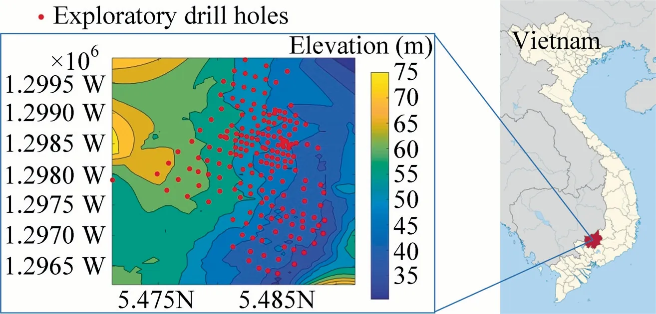
Fig.1.Locations of the study area and exploratory drill holes.
3.2.Data set
Data from 194 exploratory drill holes arranged in a grid with an average spacing of 50 m×50 m to 100 m×100 m were available for this research.Along the drill holes,the study obtained 3,877 samples and composited them into 888 data at a length of 10 m(with a minimum length of 2 m),with information on the common rock types and the six primary chemical grades,including CaO,SiO2,Al2O3,Fe2O3,MgO,and LOI (loss-on-ignition).Fig.2 shows a perspective view of the rock types and six grades in the study area.Fig.3 displays bimodal distributions of the primary chemical grades via histograms,suggesting that the data is a mixture of various populations.CaO,MgO,and LOI are mostly available in the limestone,while SiO2,Al2O3,and Fe2O3are in the remaining rock types.Table 1 shows a strong influence of rock types on the average grades.Laterite is the primary source of high grades of Al2O3and Fe2O3,and clay and limestone mainly produce high grades of CaO and SiO2,respectively.These facts motivate the resource to a hierarchical simulation approach in which modeling the rock types first can improve the accuracy of grade estimation.
4.Application of hierarchical simulation
4.1.Rock-type simulation
4.1.1.Trend modeling
Soil,clay,laterite,and limestone in the deposit show clear upward geological trends.In this study,the authors established the upward trends by splitting the composited rock type data into cells of the grid to be used in the simulation,and then,calculating the proportion of the rock-type in each cell.The authors also produced the areal trends by grouping the composited data in different regions of the study area and averaging facies proportion in each region.Nevertheless,the indication of the areal trend of rock-types is not clear.Hence,only the upward trends for rocktype simulation were considered.Fig.4 shows rock-type proportions along the vertical direction,which indicates trend as the expectation of geologists:more of limestone and less of soil,laterite,and clay are at the bottom.Matlab Curve Fitting Toolbox was used to fit the upward trend.
4.1.2.Variogram analysis
The direct variograms were computed on the codified 0–1 indicator values.First of all,2D variogram maps,which are a collection of experimental variogram values,were built to determine major horizontal directions of continuity(Fig.5).For each rock type variable,two variograms in the horizontal plane,and one variogram in the vertical direction were calculated and modeled.Finally,all experimental variograms were modeled by selecting structure types,and correlation ranges for each structure.Fig.6 presents the experimental variograms of the rock types and their fitting models in the horizontal and vertical directions.
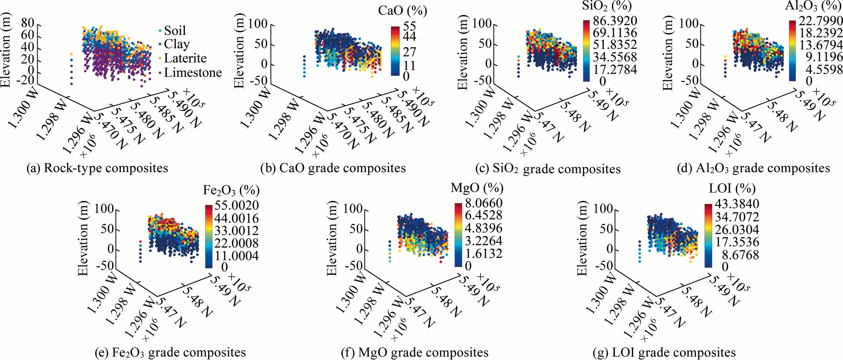
Fig.2.A perspective view showing composites of rock-type and the six grades in the study area.
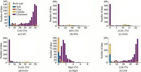
Fig.3.Histograms of the six chemical grades.

Table 1Relationships between the rock-type domains and average grades.
Table 2 shows the indicator variogram parameters for each rock type.In all rock types,the variograms have a more extensive range in the horizontal plane than along the vertical direction,which can be explained by the deposition of rock types in thin layers.The experimental variogram of soil corresponds to zonal anisotropy,where only the horizontal directions contribute fully to the total variance of the phenomenon at that scale.It is because soil mainly appears in a thin layer so that its data is insufficient to calculate the total variability.A visual representation of the experimental variograms suggests that the spherical models are reasonably in agreement with the data.
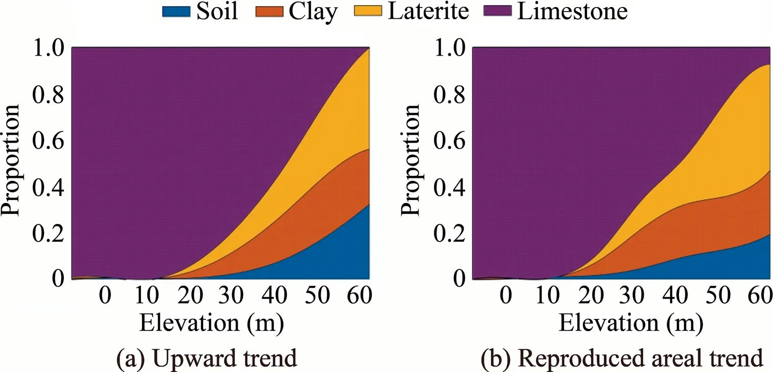
Fig.4.Rock-type proportion along the upward direction and example of reproduced trend of rock-type domains on a realization.

Fig.5.Variogram maps of soil,clay,laterite,and limestone.The red lines show the direction of maximum continuity in composited rock-type data.
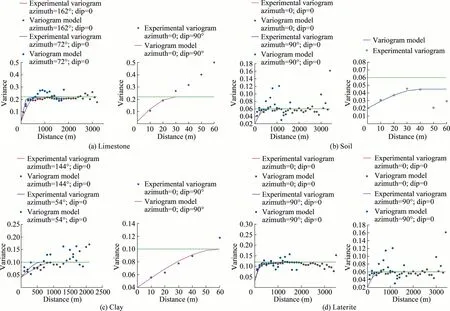
Fig.6.Experimental variograms and their suitable models in the horizontal and vertical directions.

Table 2Indicator variogram parameters for each rock type.
4.1.3.Rock-type simulation
Section 4.1.1 shows a clear trend of rock-type data along the vertical direction.Hence,constraining SIS to the trend is essential.One can decompose the rock-type data into a residual,and a locally variance mean (LVM),and use either of them to incorporate the trend into SIS.However,working with residuals may lead to some problems,including the presence of bias in the covariance matrix due to the form of trend function [12–14].In this study,the LVM was used as ancillary information that indicates a trend or nonstationary influence of the rock-type variable to simulate rock types.The simulation was performed using the sisim_lm in GSLIB software.Twenty conditional simulations of rock types were generated on block dimensions of 50 m × 50 m × 10 m,which are based on the dimension of selective mining unit sizes for the future mine planning.
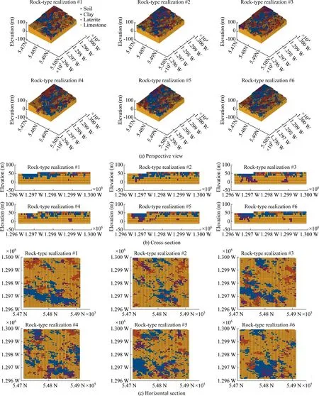
Fig.7.Perspective view,cross-section (easting=548,110 m),and horizontal section (elevation=32.2 m) of rock-type realizations.
As an illustration,Fig.7 displays the spatial distribution of four rock-type domains on six example realizations suggesting that the dominant rock type domain in the study field is limestone.The uncertainty of rock-type distribution can be accessed.For example,Fig.8a-c map the probabilities of occurrence of four rock types on 3D block models,cross-sections,and horizontal sections,respectively.In these probability maps,the yellow regions indicate a high possibility for a rock-type occurrence at these locations,while the blue areas are associated with a low chance of finding that rocktype at these locations.It is clear that the probability of the existence of limestone increases along with the depth,especially under 20 m,the limestone is very abundant in comparison with other domains,which mainly concentrate in the upper region.Realizations and occurrence probability of rock types at distinct elevation(32.2 m),as shown in Fig.8b and c,respectively,suggest that the distributions of soil,clay,and laterite are not local,concentrates in small quantities across the section,indicating the difficulty for extracting the raw materials selectively.
4.1.4.Validation
A first validation consists of a visual check of histogram and trend reproduction of rock-type domains between the realizations and the composited rock-type data:each realization should reproduce similar statistical properties and upward trends of the composited rock-type data.The reproduction of trend and histogram can be seen clearly in Figs.3 and 9,respectively.
A second validation consists of checking the ability of the simulated realizations to preserve the spatial features of the composited rock-type data during the simulation process,which can be done by comparing the fitting variogram models and the variograms on simulated data.The simulated variograms (Fig.10) are not as well-behaved and show a higher variance against the variogram model.This limitation of SIS is due to the fact that it only accounts for direct indicator variograms and ignores crossvariograms which convey information on the geometry of the domain layouts and their contact relationships as well as higherorder distributional properties.An alternative indicator simulation approach,such as plurigaussian simulation,should be considered in the future.
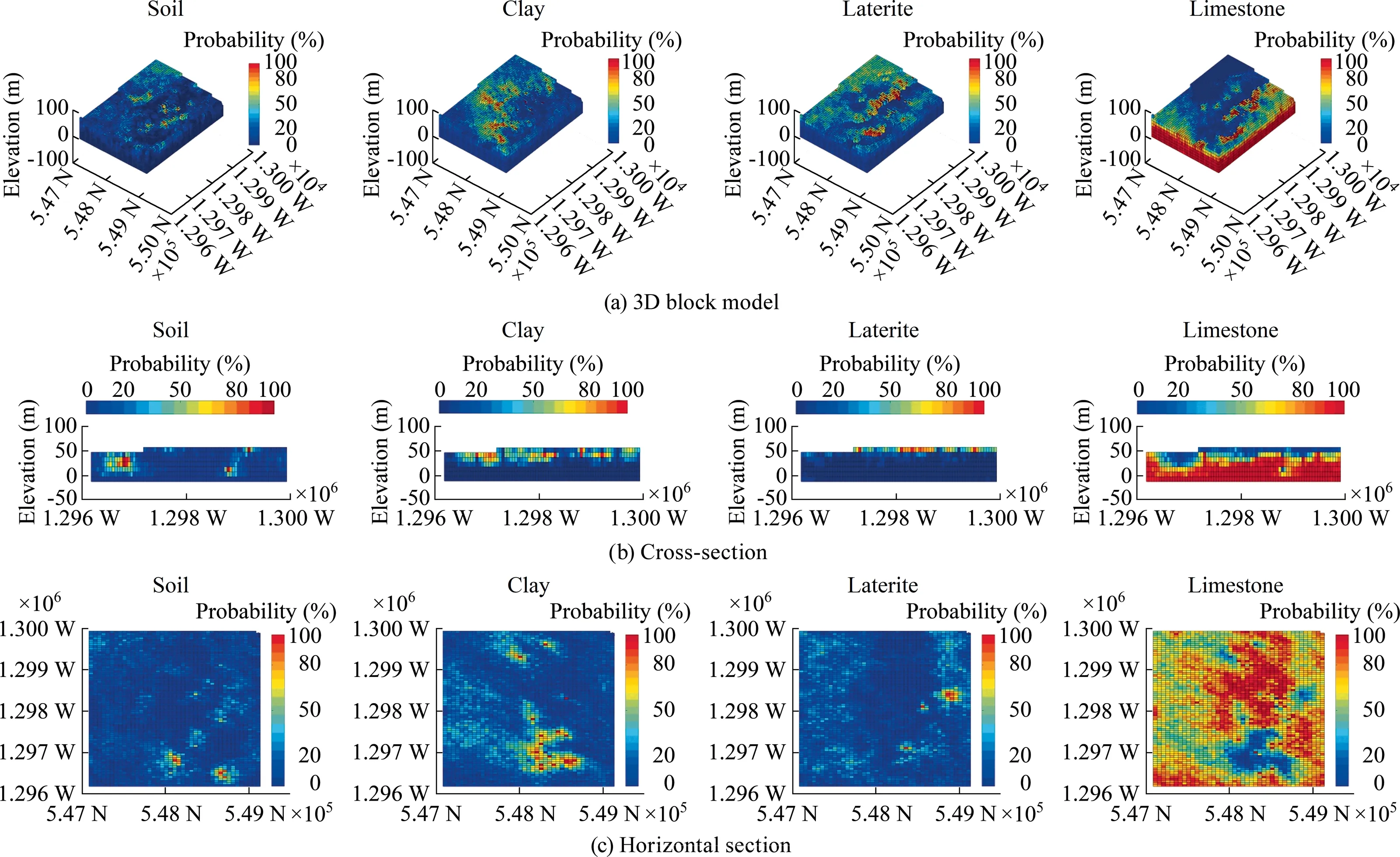
Fig.8.Probabilities of occurrence of four rock types,obtained from a set of 20 conditional realizations on 3D block model,cross-section(easting=548,110 m),and horizontal section (elevation=32.2 m).

Fig.9.Reproduced histogram of rock types between composited data and Realization #1.
4.2.Grade simulation
Based on the analysis of the data set in Section 3.2,one observes that the distributions of the grade variables are different with that of the rock types,suggesting that it is reasonable to separate the deposit into two domains for all grade variables before the resource evaluation process:the first one consists of soil,clay,and laterite (Domain 1),and the second one consists of limestone(Domain 2).
4.2.1.Grade simulation process
The grade simulation can be proceeded as follows:
(1) Cell declustering:This step is used to avoid nonrepresentative sampling in the study field.The application of cell declustering technique to the grade data set in each domain was made by declus program in GSLIB using the minimum size of 50 m,the maximum size of 100 m with the number of cell sizes,and the number of origin offsets is 50 and 5,respectively.The changes in mean values of the grades in each domain before and after declustering are shown in Table 3.
(2) Normal scores transformation:This step is used to transform the declustering data into Gaussian space or normal score before variography.
(3) Variogram analysis:In this step,2D variogram maps were generated firstly to evaluate the existence of spatial anisotropy and determine the direction of maximum continuity of Gaussian grades in each domain (see Figs.11 and 12).Experimental variograms and their fitting models were built to characterize the spatial correlation structures of Gaussian grades within their controlled domains(see Figs.13 and 14).Table 4 presents a summary of the fitting variogram models.
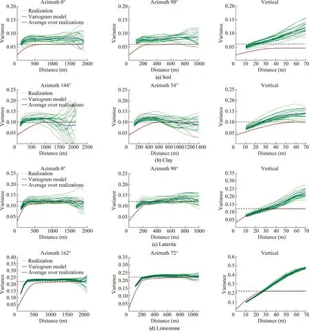
Fig.10.Reproduced variograms of four rock types.
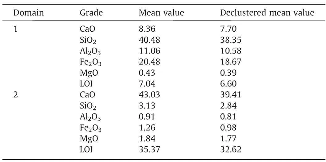
Table 3Mean values of chemical grades before and after declustering.
(4) Sequential Gaussian simulation:SGS was used to construct 20 realizations on a block size of 50 m × 50 m × 10 m for each Gaussian grade based on each of 20 rock-type layouts.To address the issue of volumetric support of blocks,we first simulated the entire domains at point support of 25 m × 25 m × 5 m,followed by averaging 20 realizations to obtain block support simulation.Since the simulation was carried out on Gaussian data,the estimated values were back-transformed to the original unit.Fig.15 shows an example of the spatial distribution of SiO2,CaO,Al2O3,Fe2O3,and MgO grades generated on rock-type Realization#1 through the 3D block model,horizontal and vertical section of the deposit.
4.2.2.Validation
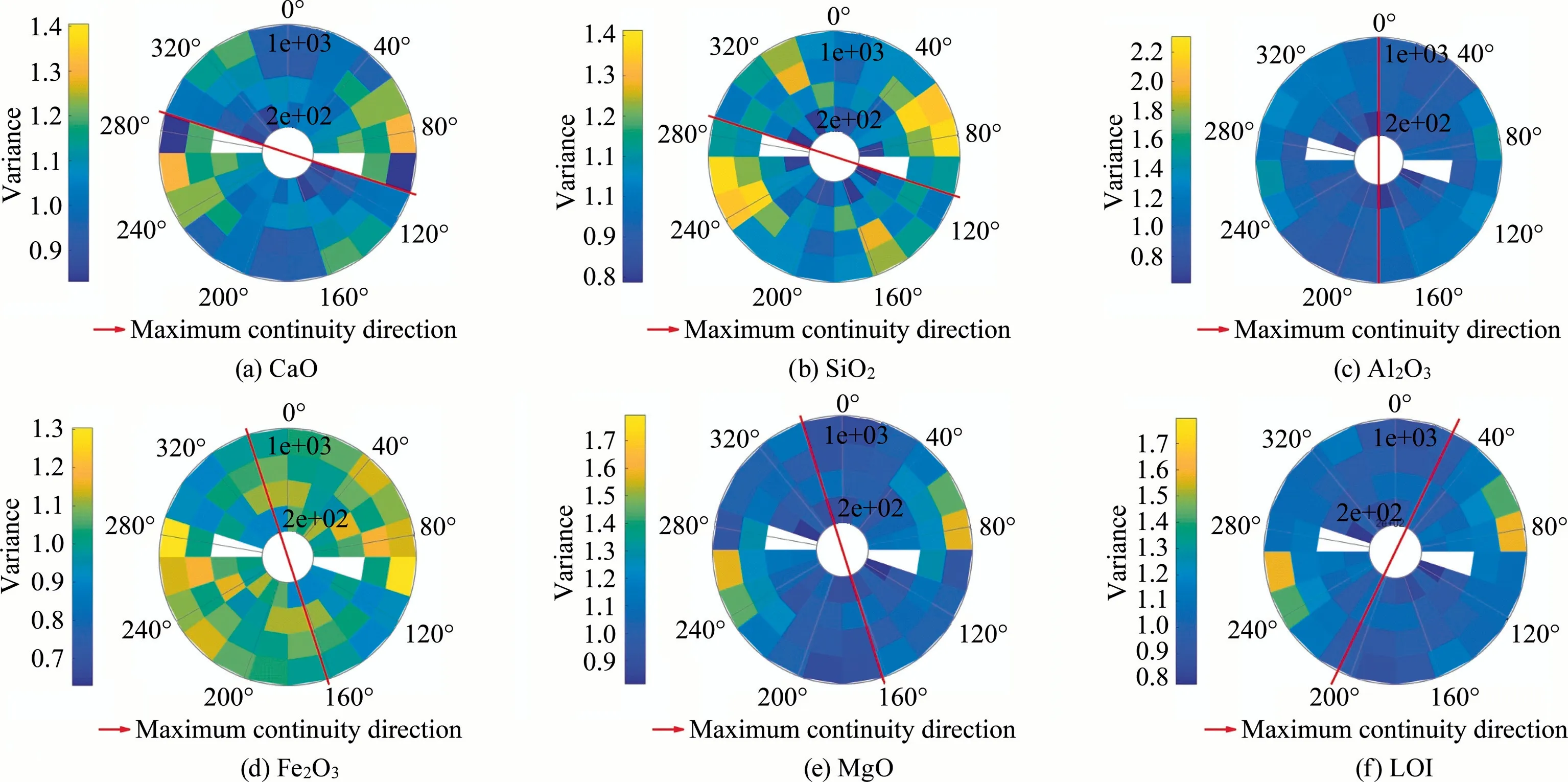
Fig.11.Variogram maps of the six chemical grades within Domain 1.The red lines show the direction of maximum continuity in composited grade data.
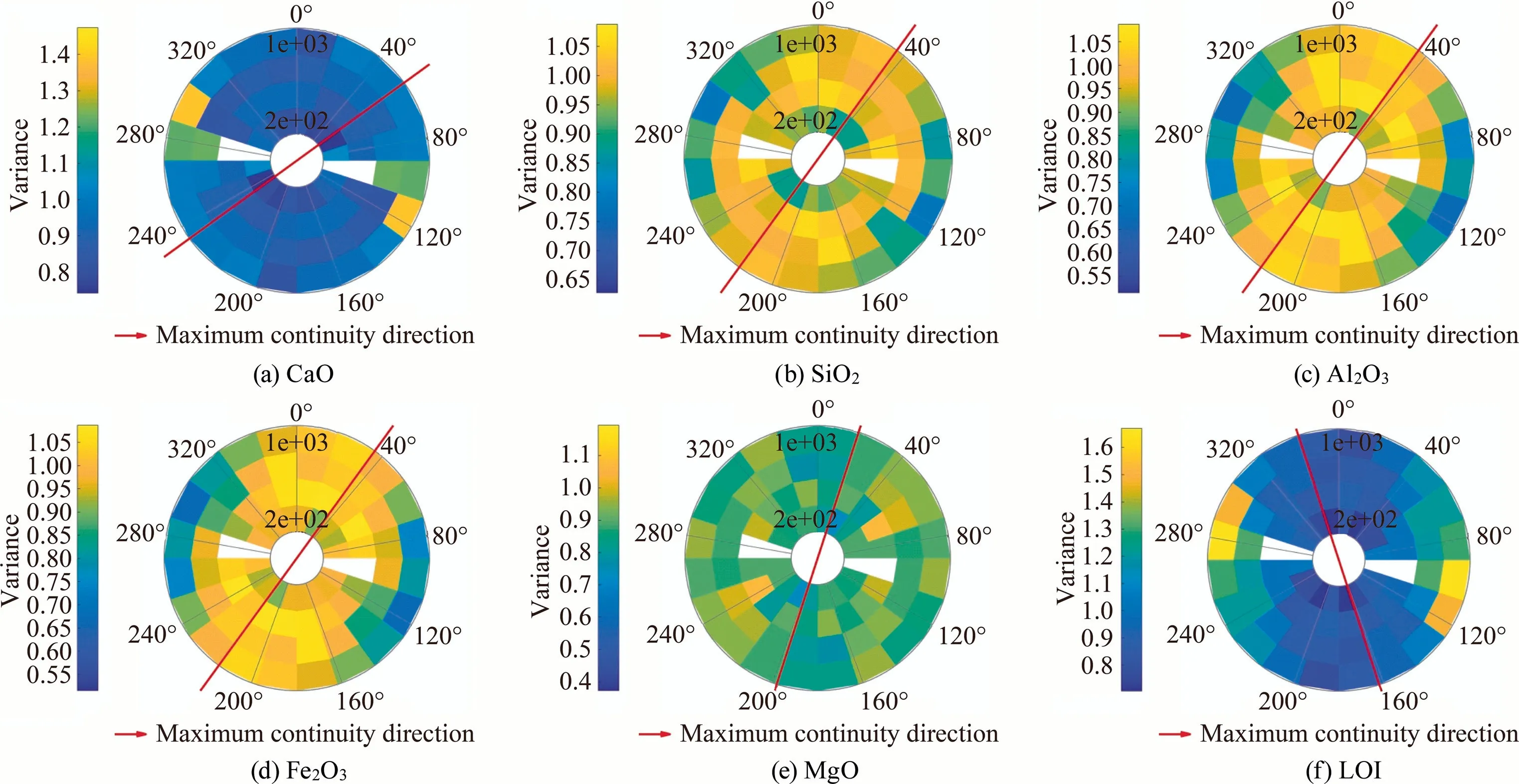
Fig.12.Variogram maps of the six chemical grades within Domain 2.The red lines show the direction of maximum continuity in composited grade data.
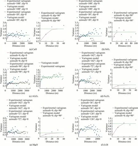
Fig.13.Experimental variograms and their fitting models of the six chemical grades in the horizontal plane within Domain 1.
Several validation checks were performed to access the results of the grade simulations.Validation consists of the visual examination of the consistency of grade distribution with the rock-type domains,the correlation between simulated grades and composited data(after declustering),and verification of histogram,experimentalvariogramreproductionofcompositeddata characteristics.Fig.15 shows the consistency between the chemical grades and the Realization #1 of rock-type domains (Fig.7),in which the grades exhibit the spatial continuity within their controlled domain and discontinuities near the boundary between Domain 1 and Domain 2.Figs.16 and 17 validate the reproduction of simulated data of the six chemical grades on the declustered data.Whereas Figs.18 and 19 present the histograms from the simulated realizations of the grades and,then,compare to the histogram of the declustered data.Also,to examine the statistical parameters,Figs.18 and 19 are prepared for simulated and declustered data of CaO grade.All comparisons suggest that the reproduction of the original data characteristics by SGS is excellent.
5.Discussion
As indicated in Section 3.2,the challenge in modeling the deposit in this study is the complexity in the geometry of the lithology,where the rock type domain is a significant factor controlling the occurrence and spatial distribution of mineral grade.The construction of the resource model without this relationship can be impractical.The left plane of Fig.20 shows the expected CaO grade(calculated based on a set of 100 CaO grade realizations)constructed without rock-type control.The distribution of CaO grade,in this case,is unreasonable.The high CaO grade appears in the regions where soil,clay,and laterite(Domain 1)have a high probability of occurrence (Fig.8).On the contrary,the approach using deterministic rock-type modeling generates the model with the expected CaO grade consistent with the structure of the rocktype domain (the middle plane of Fig.20).The grade distribution shows clear-cut discontinuities when crossing the boundary between a high-graded domain (Domain 2) and a low-graded domain (Domain 1).Although this approach relies on an interpretation of the available drill hole data,its limitation is likely to misclassify the real rock type domain due to the dependence on the subjective interpretations of geologists.As a result,errors in the rock-type modeling impact on predicted grades and tonnages.For example,limestone regions (high CaO) can be wrongly assumed to be soil regions (low CaO) or vice versa.
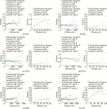
Fig.14.Experimental variograms and their fitting models of the six grades in the horizontal plane within Domain 2.
In this study,a hierarchical simulation method has been proposed to overcome this challenge,based on the stochastic rocktype modeling and,subsequently,mineral grades in each rocktype domain.SIS,which was constrained with LVM to reproduce the trend of each rock type,was chosen to simulate the uncertainty of the rock-type domain,which can generate a soft rock-type layout.The case study demonstrated the straightforwardness of this approach in transferring uncertainty in rock-type domains through the construction of 20 different numerical realizations and particularly,removing the dependence of grade model on the interpretations of geologists about the boundaries of rock-type.Despite that,there are some criticisms on SIS,such as unable imposing contact relationships amongst rock types [10] or simulation only based on two-point statistics.The right plane of Fig.20 shows the expected models of CaO grade conditioned on such 20 rock-type realizations.The clear-cut discontinuity of the grades is no longer apparent and smoother because the grade model accounts for the uncertainty in the spatial extent of rock-type domains.The stochastic rock-type modeling approach accounts for the errors of the misclassification of rock-type domains.
Ta Thiet deposit in this study was investigated to operate a cement plant,which is a significant supplier of Portland cement in southern Vietnam.The deposit consists of four main rock types,as mentioned above,in which the soil aims to strip and stockpile for use in the rehabilitation of the quarry,although we can use this material for the raw mix.The success of cement plant operation is possible only if the raw mix with optimum composition at the desired quantity is consistently supplied.The factory requires the percent content of the principal oxides,including CaO,SiO2,Al2O3,and Fe2O3should be kept within the desired limits of 40%to 45%,10%to 28%,2%to 10%,and 0%to 5%,respectively.The pre-liminary quality tests,summarized in Table 1,and the analysis of grade-tonnage curves (Figs.21 and 22),prove the suitability of the clay,laterite,and limestone in supplying raw material for the cement project at the desired limits.Besides,the factory requires a balance of the principal oxides to develop an acceptable raw mix for cement manufacturing.Lime saturation factor (LSF),silica ratio (SR),and alumina modulus (AM) are usually used to achieve the balance of the principal oxides.These indices are presented as[15]
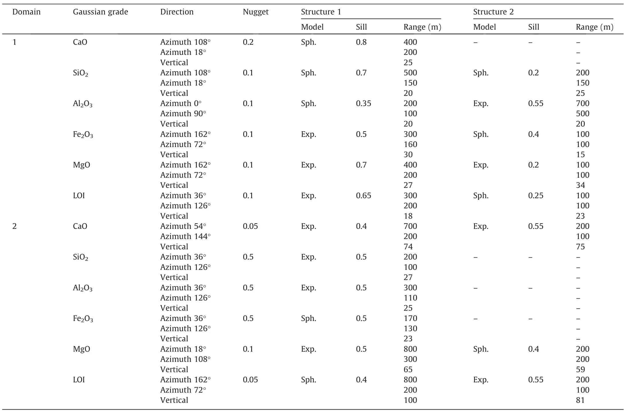
Table 4Fitting parameters of variogram models for each Gaussian grades in each domain.

For limestone rock type,LSF,which should lie between 0.85 and 1 [16],helps to achieve the balance between CaO and SiO2,Al2O3,and Fe2O3.Due to the high LSF factor through the range of CaO cut-off (Fig.21a),the limestone cannot be used independently for cement manufacturing and would require a blending of argillaceous material such as clay to arrive at suitable LSF,based on Eq.(1).The clay rock type contains a comparatively high content of SiO2and Al2O3,and a small amount of CaO,which makes it essential for manufacturing high strength Portland cement,as shown in Fig.22a-f.However,due to the low Fe2O3in the clay rock type,the expected AM and SR indices are very high in compared with the requirement of 2.6 to 2.9,and 1.5 to 3 [16],respectively,which can be corrected by adding an amount of high Fe2O3raw materials such as laterite or iron ore as shown in Eq.(2).In contrast,one can use the laterite as a source of Fe2O3for the raw mix,but it is potentially necessary to mix with silica minerals like clay,sand,or bauxite to increase the AM and SR indices in the raw materials(Fig.22g and h).MgO is another critical component that may decrease the efficiency of the manufacturing process when its concentration is above 2.5%.The limestone,clay and laterite rock types have low expected MgO grades (Fig.21b,and Fig.22c,f and i),which they are suitable for cement manufacturing in terms of acceptable MgO grade.Only a small tonnage of limestone has an expected MgO higher than 3.5% when CaO increases more than about 53%.
6.Conclusion
In Ta Thiet cement raw material deposit,the structure of rocktype domains is quite complicated and required to separate from each other in the resource evaluation stage,making difficulties for geologists to interpret their layout.Also,the application of the deterministic modeling approach often fails to qualify the uncertainty in the occurrence of each rock-type domain,which may produce a significant error in grade model construction.The proposed hierarchical approach successfully solved this problem,based on probabilistic simulation of the rock types,and then combining the rock-type layout simulations with the grade simulation within each rock type.The simulation results of the rock-type and chemical grades also support the assessment of the related risk through the range of realization outcome and the grade-tonnage curves.The analysis of risk suggests the suitability of clay,laterite,and limestone in the cement manufacturing process,and the blending is necessary to achieve the balance of the primary oxides.Finally,the simulation results allow transferring uncertainty of both rock-type domains and grades into risk in downstream processes.
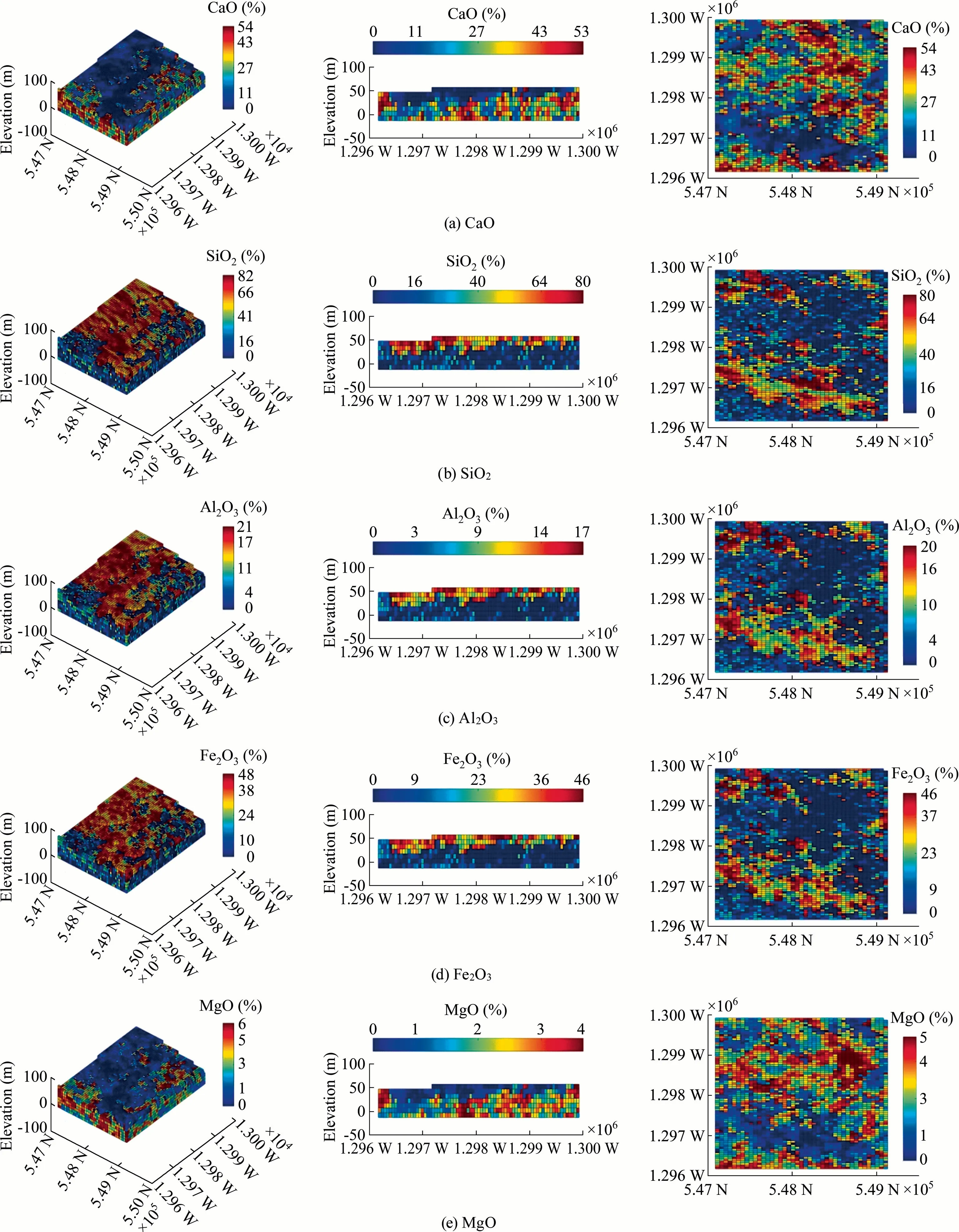
Fig.15.Example of the spatial distribution of CaO,SiO2,Al2O3,Fe2O3 and MgO grades generated on rock-type Realization #1 on 3D block model (left plane),cross-section(easting=548,110 m) (middle plane),and horizontal section (elevation=32.2 m) (right plane).
The proposed approach is robust and able to acquire the available conditioning data at sampling locations,including trend,statistical characteristics,and spatial variability.However,the effect of using SIS must be understood in terms of poor reproducing rock-type geometry.Besides,the application of SGS in this study ignores the presence of correlations between variables of interest,such as CaO and LOI.Future work should,therefore,investigate the correlation and consider the application of joint or co-simulation techniques to improve the reality of the simulation.
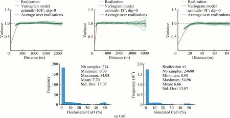
Fig.16.Variogram and histogram reproduction in the three main directions of the six chemical grades within Domain 1.
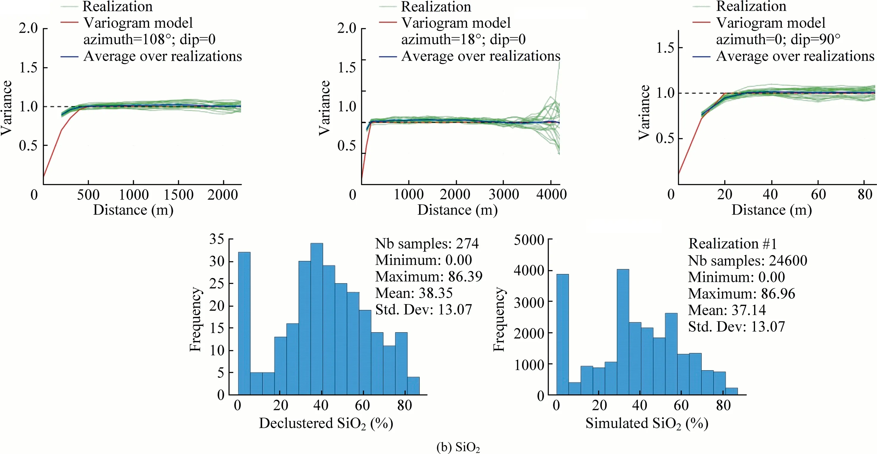
Fig.16(continued)
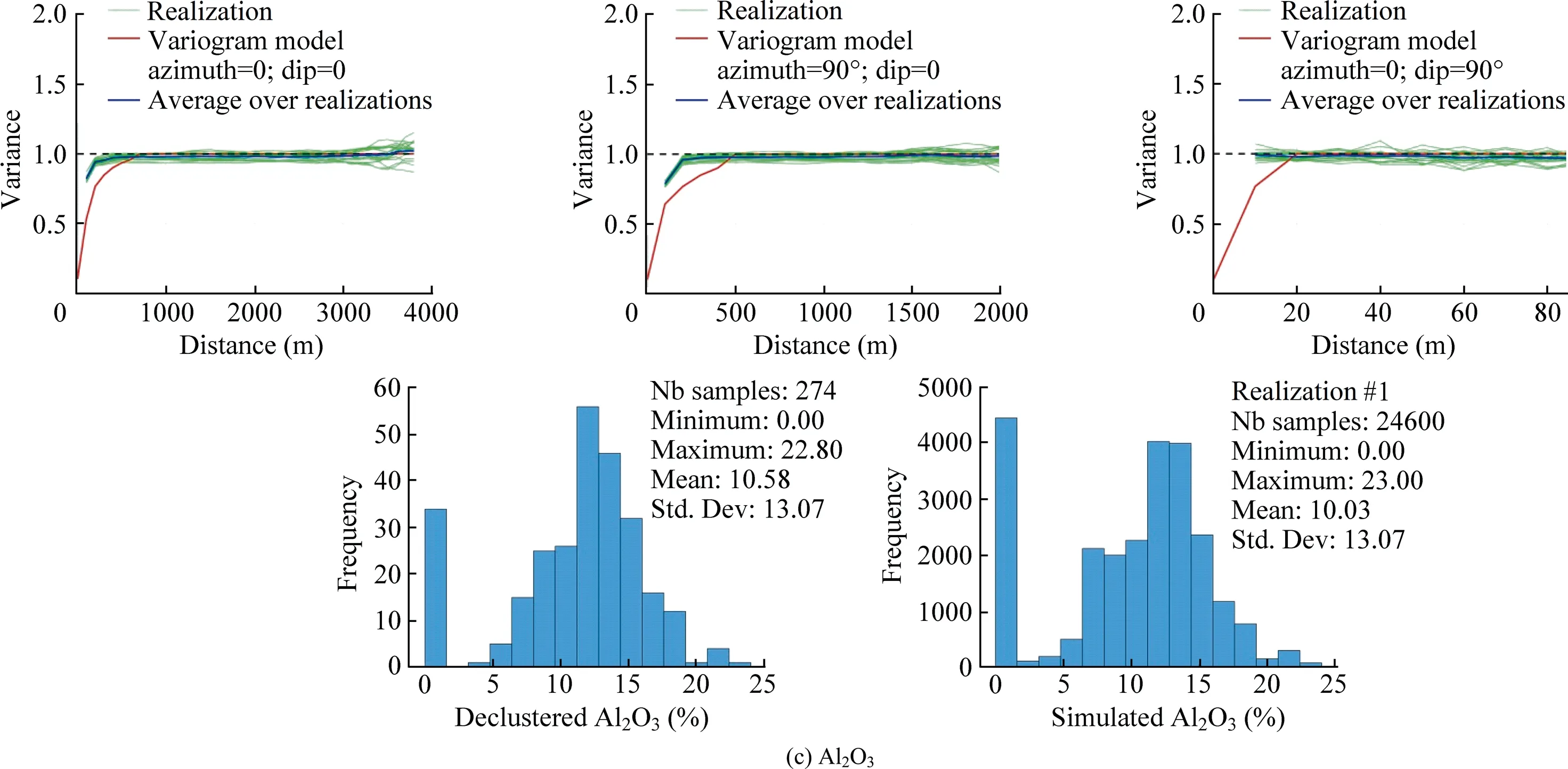
Fig.16(continued)
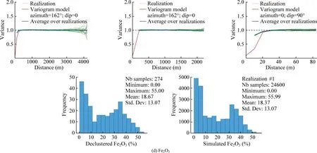
Fig.16(continued)
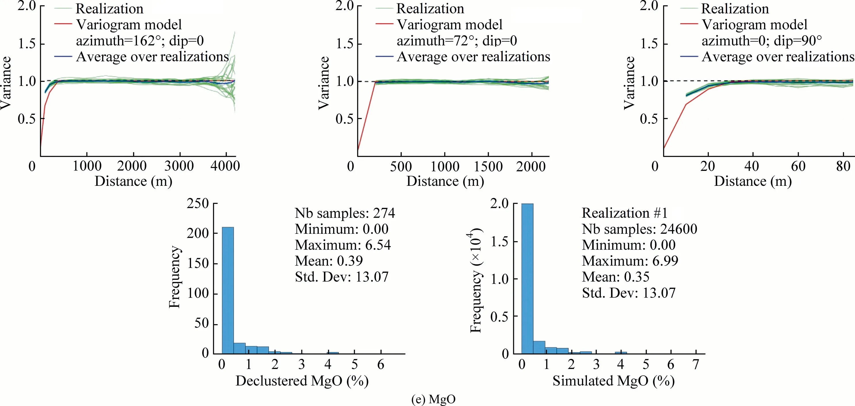
Fig.16(continued)
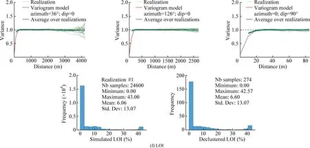
Fig.16(continued)
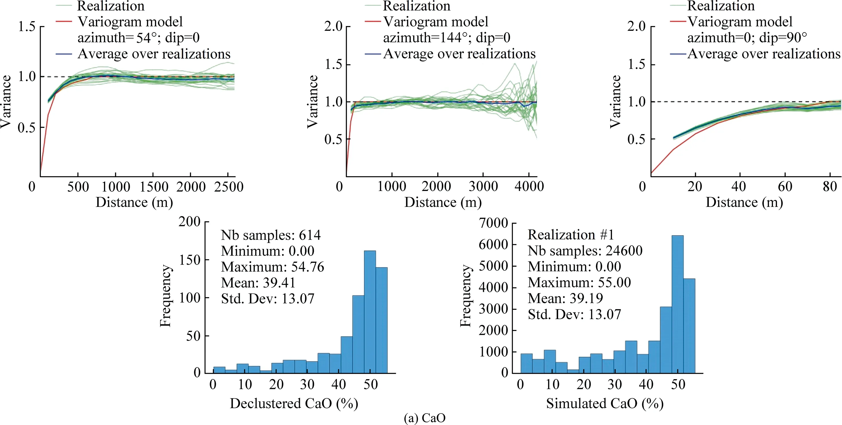
Fig.17.Variogram and histogram reproduction in the three main directions of the six chemical grades within Domain 2.
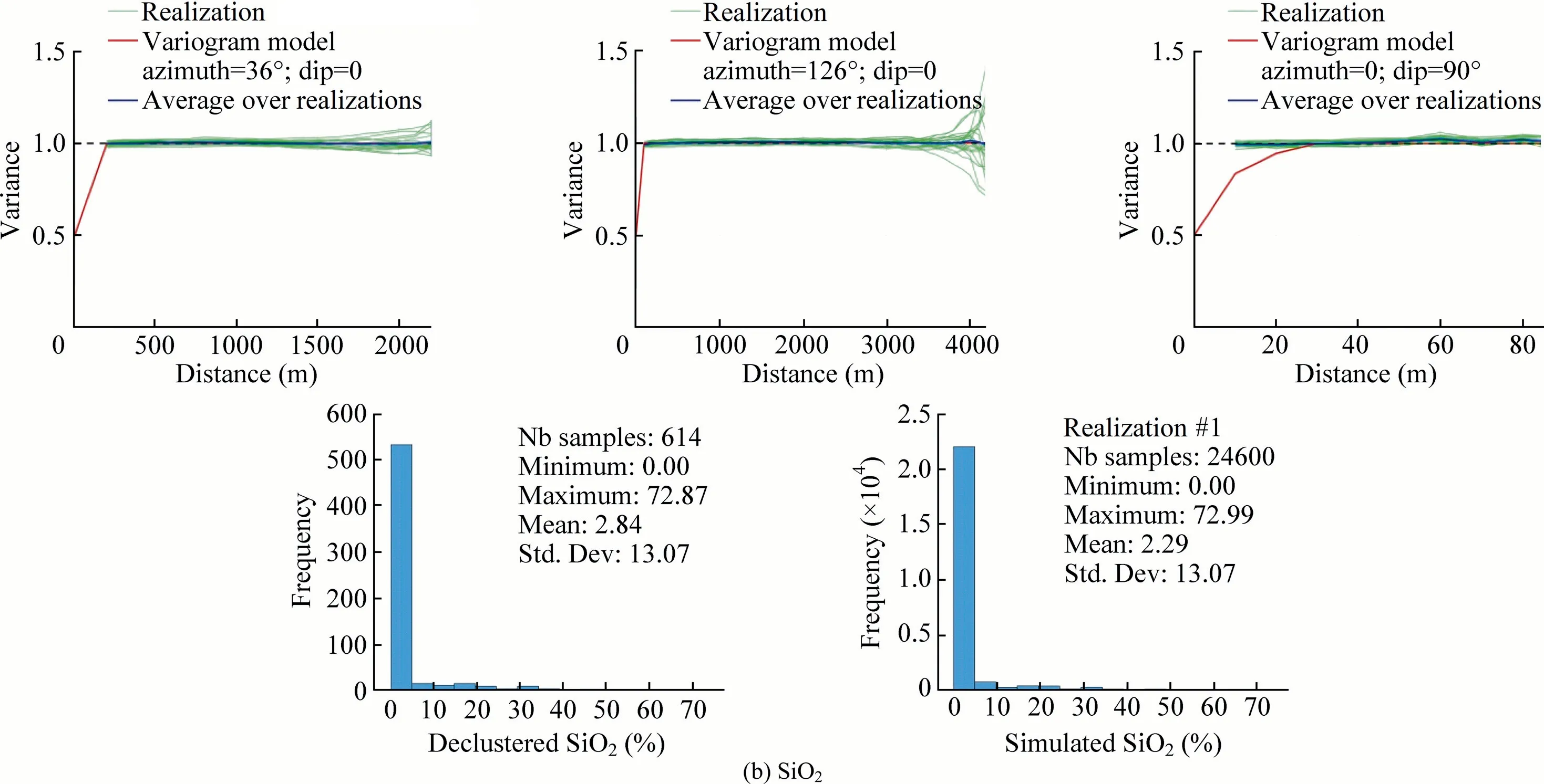
Fig.17(continued)
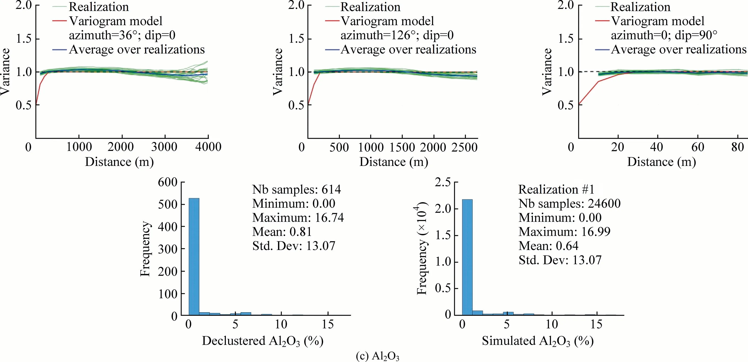
Fig.17(continued)
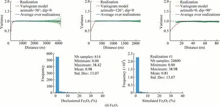
Fig.17(continued)
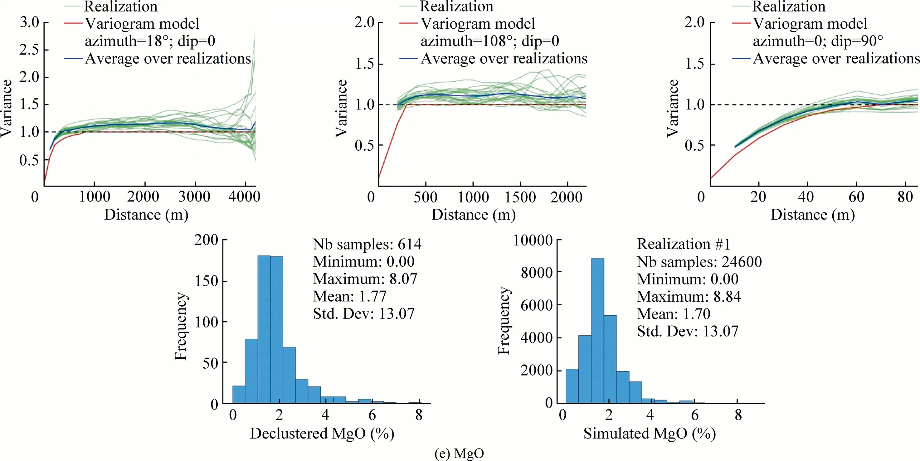
Fig.17(continued)
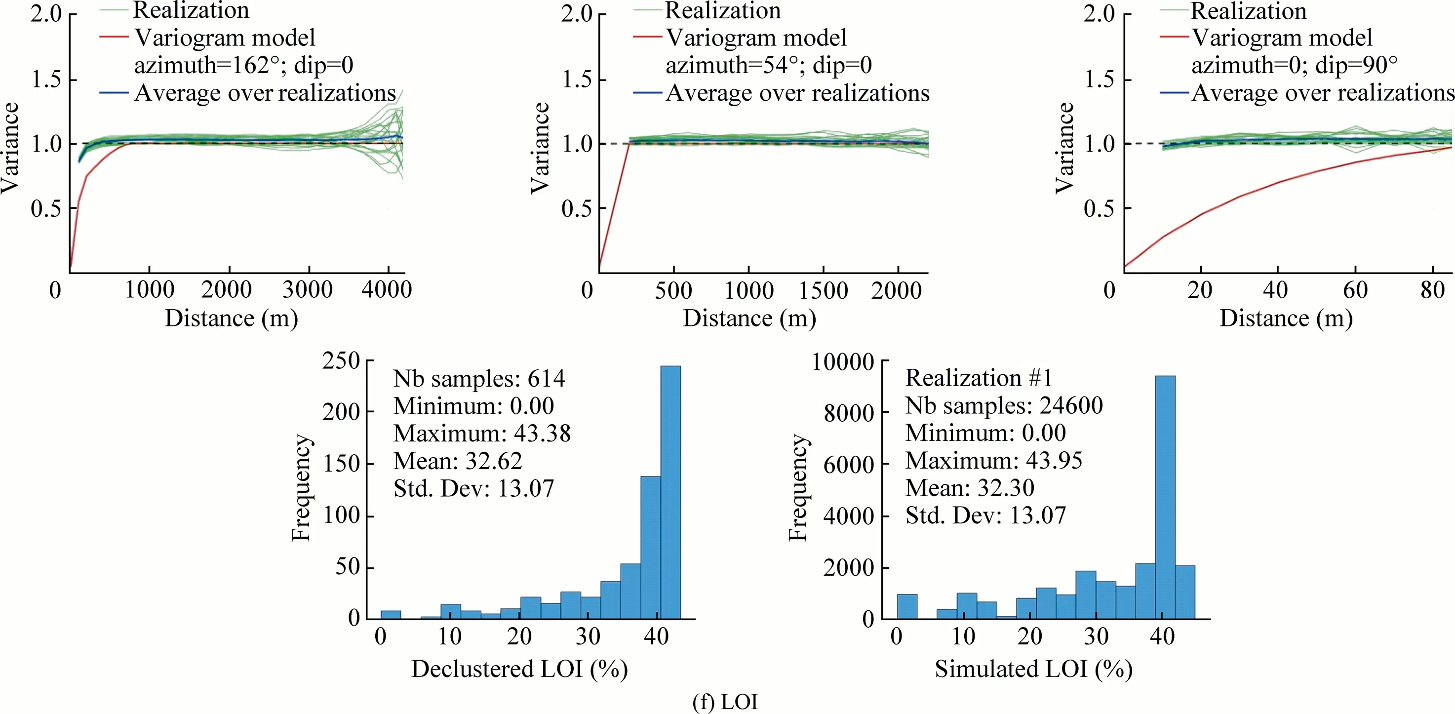
Fig.17(continued)
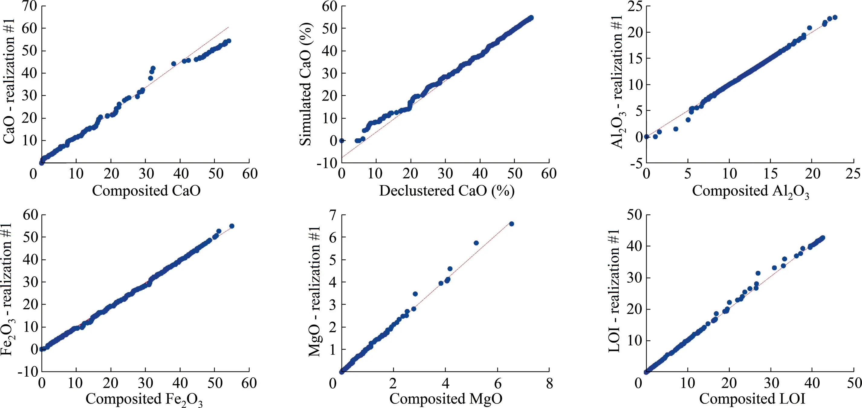
Fig.18.Q-Q plot of the six chemical grades versus their declustered data in Domain 1.
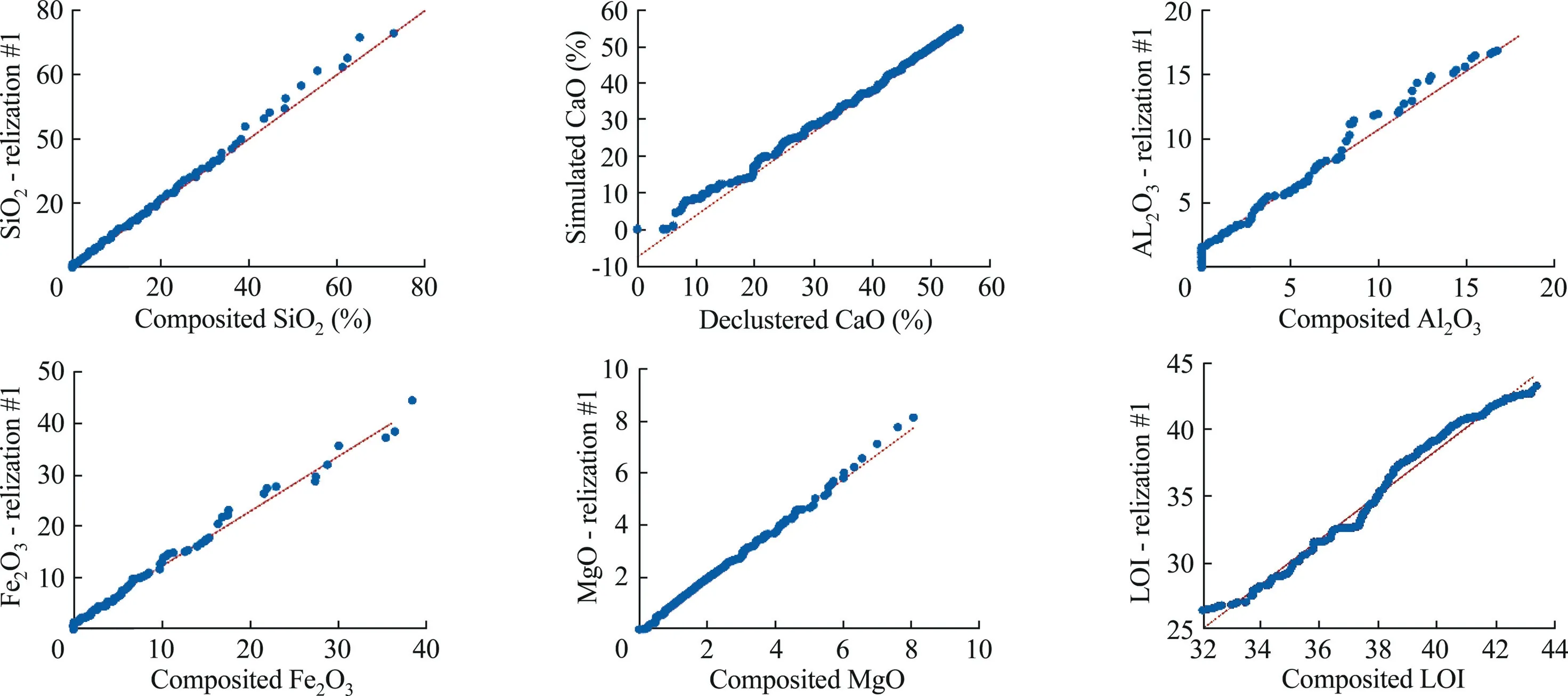
Fig.19.Q-Q plot of the six chemical grades versus their declustered data in Domain 2.
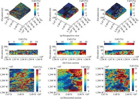
Fig.20.Perspective view,cross-section (easting=548,110 m),and horizontal section (elevation=32.2 m) of the expected CaO grade (calculated by averaging the 20 realizations of chemical grades),obtained without rock-type modeling (left plane),with deterministic rock-type modeling (middle plane),and with stochastic rock-type modeling (right plane).
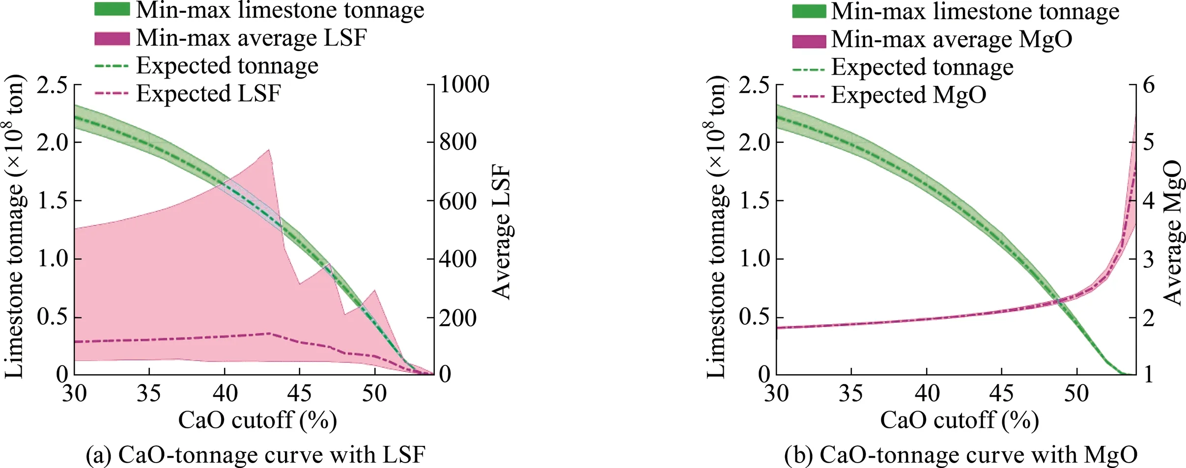
Fig.21.Simulations of recoverable tonnage with average LSF and MgO as a function of CaO cut-off (calculated over 100 realizations).
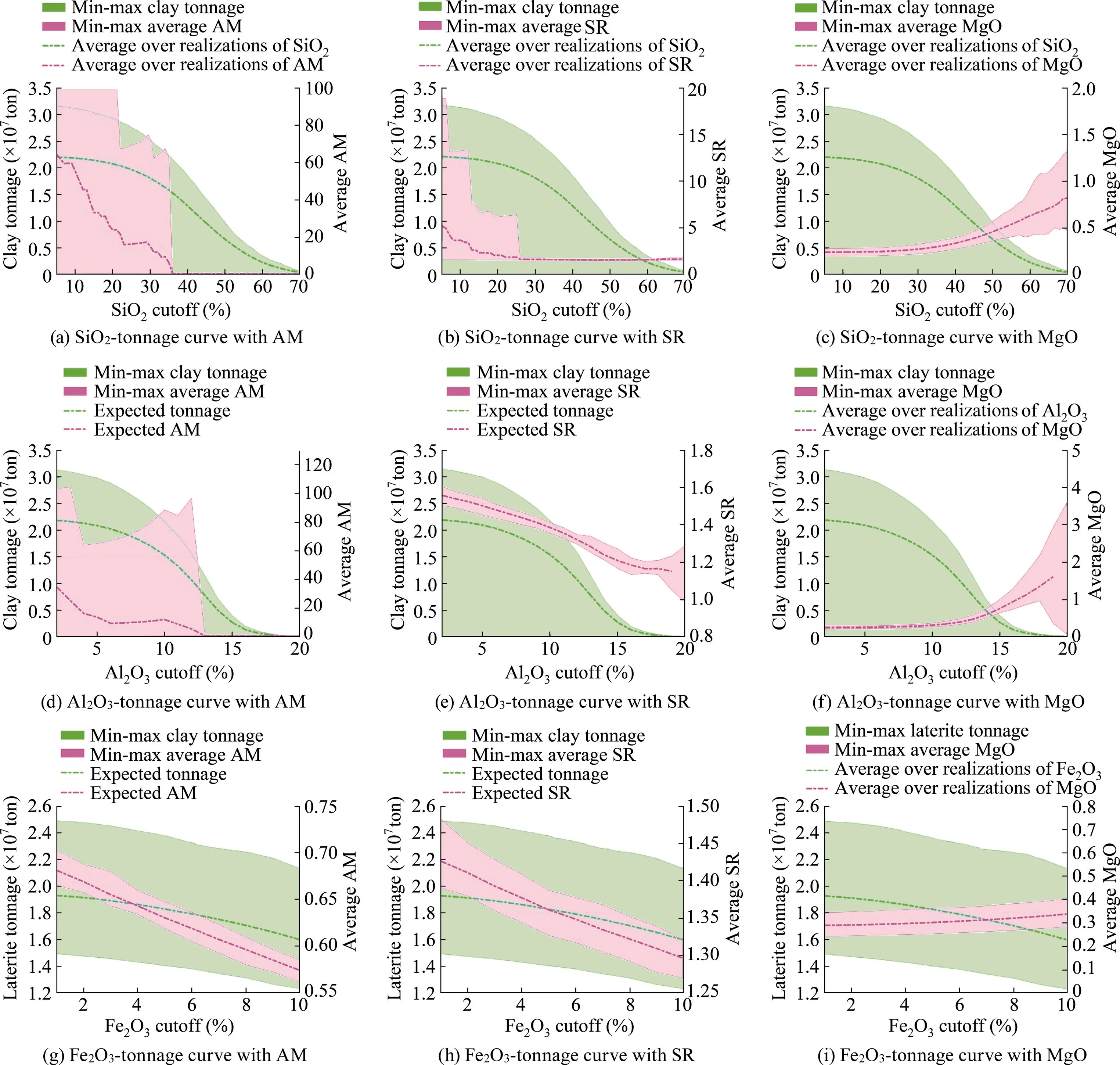
Fig.22.Simulations of recoverable clay tonnage with average AM,SR,and MgO as a function of SiO2 and Al2O3 cut-offs,and recoverable laterite tonnage with average AM,SR,and MgO as a function of Fe2O3 cut-off respectively (calculated over 100 realizations).
Acknowledgement
The authors would like to extend their sincere gratitude to Binh Phuoc Cement Factory Administration for providing data for this study.
杂志排行
矿业科学技术学报的其它文章
- Identification of digital technologies and digitalisation trends in the mining industry
- Experimental and theoretical investigation on mechanisms performance of the rock-coal-bolt (RCB) composite system
- Creep characteristics of coal and rock investigated by nanoindentation
- An experimental investigation of the fracturing behaviour of rock-like materials containing two V-shaped parallelogram flaws
- Comparative evaluation of different statistical tools for the prediction of uniaxial compressive strength of rocks
- A rapid and accurate direct measurement method of underground coal seam gas content based on dynamic diffusion theory
