Comparative evaluation of different statistical tools for the prediction of uniaxial compressive strength of rocks

Ahmet Teymen,Engin Cemal Mengüç

a Department of Mining Engineering,Nig˘de Ömer Halisdemir University,51240 Nig˘de,Turkey

b Department of Electrical and Electronics Engineering,Nig˘de Ömer Halisdemir University,51240 Nig˘de,Turkey

ABSTRACT In this study,uniaxial compressive strength (UCS),unit weight (UW),Brazilian tensile strength (BTS),Schmidt hardness(SHH),Shore hardness(SSH),point load index(Is50)and P-wave velocity(Vp)properties were determined.To predict the UCS,simple regression(SRA),multiple regression(MRA),artificial neural network (ANN),adaptive neuro-fuzzy inference system (ANFIS) and genetic expression programming(GEP) have been utilized.The obtained UCS values were compared with the actual UCS values with the help of various graphs.Datasets were modeled using different methods and compared with each other.In the study where the performance indice PIat was used to determine the best performing method,MRA method is the most successful method with a small difference.It is concluded that the mean PIat equal to 2.46 for testing dataset suggests the superiority of the MRA,while these values are 2.44,2.33,and 2.22 for GEP,ANFIS,and ANN techniques,respectively.The results pointed out that the MRA can be used for predicting UCS of rocks with higher capacity in comparison with others.According to the performance index assessment,the weakest model among the nine model is P7,while the most successful models are P2,P9,and P8,respectively.

Keywords:Uniaxial compressive strength Adaptive neuro-fuzzy inference system Multiple regression Artificial neural network Genetic expression programming

1.Introduction

Uniaxial compressive strength (UCS) is the most significant parameter used to characterize the intact rock in many engineering projects carried out in rock or soil environments(such as slope stability,rock excavation,tunnel,drilling,and dam design).Besides,UCS is one of the basic parameters used in such projects and it is also used in the rock mass rating(RMR)system and rock failure criteria.As is known,direct measurement of the UCS value of rocks requires quality intact cores with a specific geometry.Besides,it is relatively costly and time consuming to determine the UCS of rocks by applying this test defined in standards such as ISRM and ASTM.Smooth and perfectly parallel core samples cannot always be extracted from weathered,fractured,weak,foliated,thinly bedded,or block-in-matrix rocks [1].For the reasons listed above,a prediction of the UCS from simple tests (physical,mineralogicalpetrographic,index and mechanical) is economic and easy.There are many studies in literature where prediction equations are derived from simple regression (SRA) and multiple regression(MRA) techniques.Recently,in addition to traditional methods such as SRA-MRA techniques used to create prediction models in rock engineering,new techniques such as regression trees,adaptive neuro-fuzzy inference system (ANFIS),artificial neural network (ANN),and genetic expression programming (GEP) have been used to estimate the desired properties [2–23].

Gokceoglu et al.[24]carried out studies for assessing the elastic constants of rocks utilizing fuzzy logic (FL) and ANN.Gokceoglu et al.[25]developed MRA and rule-based fuzzy models to estimate the UCS of some clay-bearing rocks.Sarkar et al.[2] tried to estimate the shear strength and UCS of different rock types by using the ANN method.They used parameters such as point load index(Is50),slake durability index (SDI),density and dynamic wave velocity.Dehghan et al.[3] derived equations using ANN and regression analysis methods to estimate UCS.They used rock properties such as porosity,P-wave velocity(Vp),Is50and Schmidt hardness(SHH)test.Cevik et al.[26]analyzed the test results using the ANN method to predict the UCS of some clay containing rocks.Yagiz et al.[4] investigated the effects of the cycling integer of the SDI test on intact rock behavior.They used ANN and regression techniques to estimate major rock properties such as UCS from the index properties of rocks.According to the results of their study,rock properties such as Vp,SHH,SDI,and density can be used to estimate UCS value.A comparative study of ANFIS systems and a generalized regression ANN approach was conducted in a comprehensive article by[5].The results of the study showed that the performance of the regression ANN approach is higher than the ANFIS.Singh & Verma [27] correlated the petrographic properties and strength of schistose rocks with a comparative analysis of intelligent algorithms.According to the authors,the method can be used effectively in any situation to obtain a texture coefficient and deformation modulus from much simpler tests,which are vital for any planning and design to have better stability and safety.In their study of conglomerates,Minaeian & Ahangari [28] used simple and multivariate regression techniques to estimate the relationship between Vp,SHH and UCS.Ozbek et al.[29] used GP for predicting UCS from the unit weight (UW),water absorption(WA),and effective porosity (EP) values.

Yesiloglu-Gultekin et al.[6]used the ANFIS to predict the UCS of the same granitic rocks from the mineral contents.They could not obtain considerable relationships from SRA of these similar rocks.However,they obtained high correlation coefficients such as 0.91 and 0.87 by ANFIS and nonlinear MRA methods,respectively.Verma&Singh[30]stated that the proposed ANFIS model for estimating Vphas higher performance in modeling nonlinear,complex and multivariate problems.Armaghani et al.[7]used three nonlinear estimation tools (ANN,ANFIS,and NLMR) in their studies to estimate UCS of granites and compared their performance.They determined that the ANFIS model showed the most successful performance among these three methods.There are many studies in literature using simple MRA techniques to estimate UCS of rocks[31–43].In their study using five different rocks,Cargill&Shakoor[31] found correlations between UCS and some tests such as SHH,Is50,SDI and Los Angeles abrasion and also found that the strongest correlation was obtained by Is50testing.Singh & Singh [32] investigated the relationship between these two parameters in their studies,where they determined the UCS and Is50of quartzites.The study carried out by Tuǧrul&Zarif[33]revealed new relationships between the engineering properties of granite and petrographic properties.Using SRA,the correlation between UCS and other rock characteristics including Is50,Brazilian tensile strength(BTS),and Vpwas also investigated.Singh & Dubey [34] proposed some empirical relationships to predict the UCS of coal measure rocks by Vp.Kahraman [35] improved the relationship between UCS and practical tests such as Vp,Is50and SHH.Yang&Rosenbaum [8] developed a confidential model to control deformability and rock strength based on some mineralogical properties of sandstones.Tsiambaos & Sabatakakis [44] mentioned the existence of different factors affecting the relationship between Is50and UCS.Kahraman et al.[36] applied EP,Is50,and UCS tests to 38 rocks of sedimentary,magmatic and metamorphic origin,and determined significant correlations between these parameters.Basu & Aydın [37] determined an experimental relationship between Is50and UCS in their studies using Hong Kong granites.Çobanog˘lu & Çelik [45],taking into account the effect of core diameter,investigated the relationship between UCS,SHH,Is50and Vp.Dinçer et al.[46]developed empirical equations using some index properties and physical tests to estimate the mean tangent Young’s modulus (Et)and UCS of caliches.

Sharma & Singh [38] developed some empirical equations to estimate dependent variables such as the impact strength,SDI and UCS using the Vpindependent variable.Kahraman&Gunaydin[39]found a relationship between UCS and Is50for a data set composed of rocks of different origins with the help of regression analysis.Diamantis et al.[47]conducted statistical studies to estimate UCS using parameters such as Vpand Is50in their studies using serpentinites rocks.Basu & Kamran [40] examined the relationship between Is50and UCS with their studies on schistose rocks.Yagiz[41] performed a study predicting the rock properties such as UCS,SHH,SDI,Et,WA,EP,saturated and dry density using the most important non-destructive test method Vpvalues.It revealed a significant relationship between Vpand UCS of rocks.Sharma et al.[42] determined some equations between SHH test with SDI,Vpand impact strength index.Singh et al.[43] tested and confirmed the empirical relationship between UCS and Is50in a study using some Indian rocks.

2.Sampling and experimental studies

The rocks used in this study were collected from the factories,outcrops,and quarries in different locations of Turkey.Tests were carried out on blocks or pieces taken from fresh parts of 93 different rocks from 32 rock types (gabbro,limestone,granite,sandstone,quartzite,tuff,diabase,etc.).The class of tested rocks is composed of sedimentary (28),volcanic (20),plutonic (15),metamorphic (13),pyroclastic (10) and subvolcanic (7) rocks.The rock samples were macroscopically inspected and samples that did not have any alters and did not contain discontinuities were used.Afterward,laboratory tests including UCS,UW,BTS,SHH,Shore hardness (SSH),Is50and Vpwere carried out on those samples.The Brillant 250 wet abrasive cut-off machine was used for sizing and smoothing the core samples.During the sample preparation and testing phase,standard laboratory test procedures were used as ISRM [48] and ASTM [49] suggested.Type,class,location,and test results of the rocks are listed in Table 1.

Fig.1 shows the distribution of UCS data of 93 rock samples according to rock strength classification while Fig.2 shows the correlations and histogram graphs presenting the frequency distributions of all tests.The positive linear relationships between UCS and other features of the rocks can be seen from Fig.2.Overall,there is a meaningful relationship between some rock properties with UCS except for UW.This is also seen from the histogram graphs in Fig.2,which show the frequency distributions of the tests.It is observed that approximately half of the rocks used in the tests are in the ‘‘very high strength”,30% are ‘‘high strength” and 20%are ‘‘medium and low strength” class.

3.Constructions of models

To predict the UCS of rocks,five different techniques including simple SRA,MRA,ANN,ANFIS,and GEP have been utilized.For this purpose,the dataset developed from BTS,SHH,SSH,Is50,Vp,and UW tests of 93 different rock samples were used as input parameters for targeted models and UCS of rocks was predicted as a function of these properties.For each model (named as P1–9),two of the above-mentioned tests were used as input parameters:P1(Is50,Vp),P2 (Is50,BTS),P3 (Is50,SHH),P4 (Is50,SSH),P5 (Is50,UW),P6(Vp,BTS),P7(Vp,SSH),P8(BTS,SHH)and P9(BTS,SSH).According to McCord-Nelson& Illingworth’s recommendation (20% to 30% of all datasets can be used for testing) [50],dataset obtained from eight experiments on 93 different rock materials was randomly divided as training (70% i.e.65 data) and testing (30% i.e.28 data)subgroups by a program developed in the MATLAB environment by the authors.

To compare the findings acquired from the MRA,ANFIS,ANN and GEP techniques,identical data were utilized in training,testing and checking of the models.In order to check the validity of the models developed with the data of 93 rock,a data pool was formed with the results of the experiment of 2404 rocks collected from 87 articles in literature.For the nine equations developed using different estimation tools,the experimental results of the rocks of different origins in this data pool were used.To the checking of these nine models,260-,200-,280-,50-,240-,100-,16-,110-,and 70-piece data were used,respectively.The datasets were modeled with the help of different statistical programs and compared with each other to choose the best model.Besides,the UCS values obtained from the derived models were compared with the real UCS values obtained from the laboratory study with the help of various graphs.

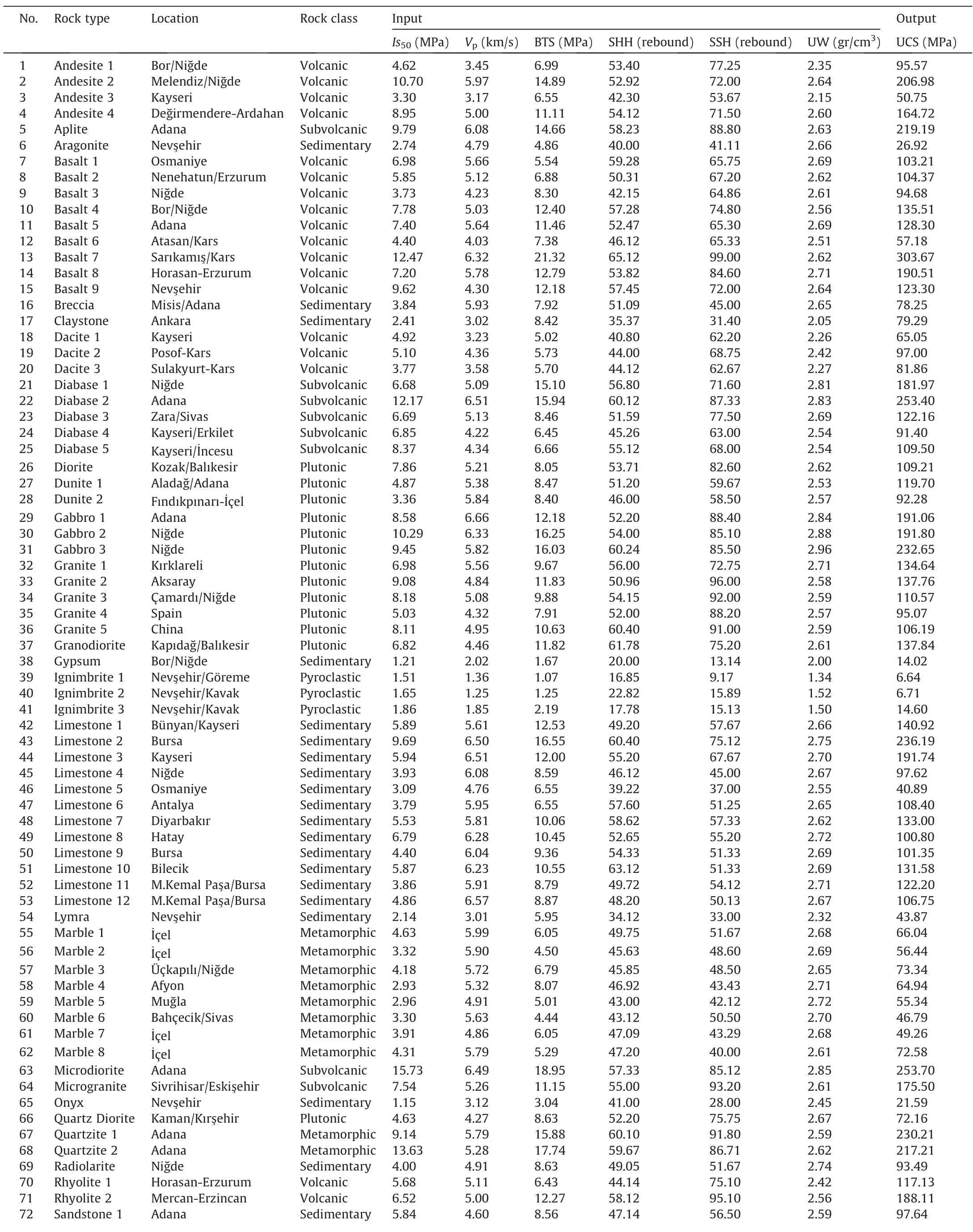
Table 1Mechanical and physical test results of the rocks.

(continued on next page)

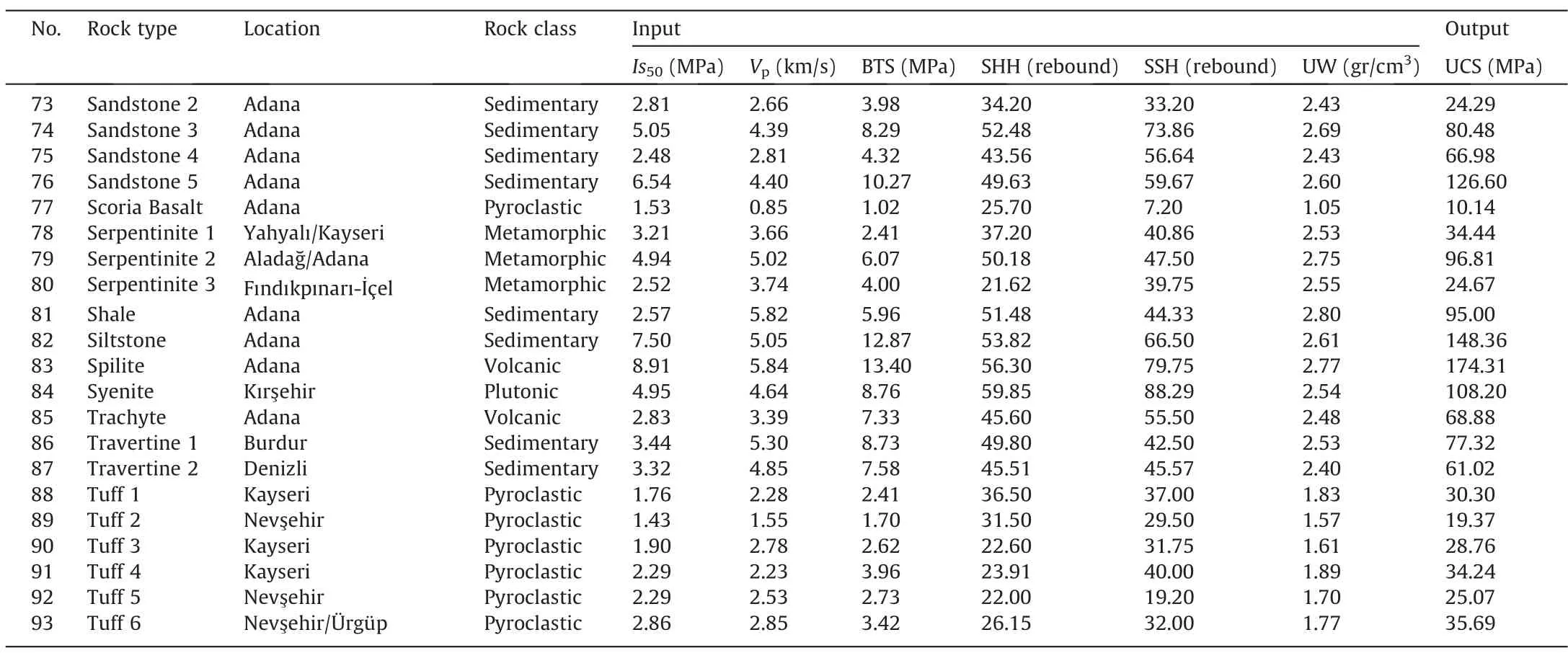
Table 1(continued)

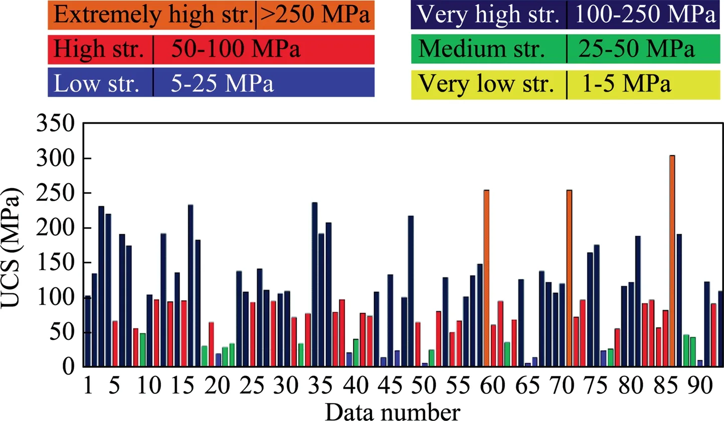
Fig.1.Distribution graph of UCS data by rock strength classification.

3.1.Simple regression (SRA)

The frequently used method to obtain estimation models between rock properties is the regression analysis,in which both SRA and MRA were used herein.In this study,first of all,SRA was performed to determine the weight of each input parameter for aimed models using the power and exponential functions.Statistical Package for Social Science(SPSS)computer package was used for SRA including F-tests and t-tests.

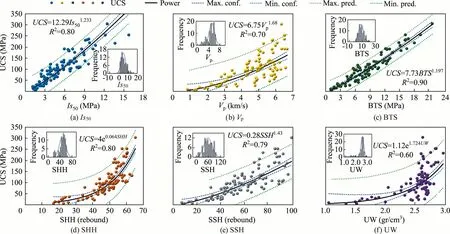
Fig.2.Histogram graphs and correlations of test data.

95% confidence interval values were calculated for the validity of the equations (see Table 2).The t-test was used to determine the significance level of the correlation coefficients of the equations and it was seen that the obtained t-values are greater than the tabulated values (1.987).It was also observed that the significance of the t-values is below 0.05 value.Regression analysis of variance was used to determine the importance of regressions.It has been seen that F-values of all equations have considerably high values than the tabulated F-values (3.95).In these equations,the correlation coefficients R2are taken into consideration to evaluate the prediction capacities of the presented equations.The R2values obtained from equations related to UCS vary from 0.60 to 0.90 for the full dataset,from 0.43 to 0.86 for the training dataset,and from 0.78 to 0.95 for the testing dataset.Derived equations that were proven to be reliable with F-and t-tests can be reliably used,especially for predictive purposes.The results obtained from simple correlations revealed acceptable and significant statistical relationships between UCS and relevant independent variables.Although these results were acceptable for estimating UCS,MRA was also performed to obtain stronger estimates.

3.2.Multiple regression analysis (MRA)

In cases where more than one independent variable can be used as input parameters,MRA can be applied to obtain the most relevant and appropriate equation.In the second phase of the regression analyses,a series of MRA was carried out using two independent variables for predicting UCS.For the development of the best regression models,the enter technique in the statistical software package of SPSS [51] was employed.All multiple regressions revealed in this study were successful at a 95% confidence level for the F-and t-test.In addition to F-and t-tests,it was also examined whether there is a multicollinearity problem (variance inflation factor,abbreviated as VIF) to perform a stronger validation in multiple regression equations (Eqs.(1)–(9),Table 3).

When the equations obtained from MRA and their reliability analyses are examined in detail,it is seen that the most reliable results and high correlation coefficients in UCS estimation can be obtained with Is50,BTS,SSH,and Vptests.When Table 3 is examined in detail,it is clear that multiple equations can be used for more accurate and strong estimations.Because MRA models include two independent variables,the correlation coefficients,and estimation capabilities are higher than that of the simple models shown in Table 2.All binary combinations of the seven independent variables were tried as input parameters.Equations that are significant and successful in terms of F-and t-test and VIF tests were taken into consideration.

3.3.Artificial neural networks (ANN)

ANN is one of the soft computing techniques that has been used in several fields of technology and science since the 1940 s and inspired by the human brain information process.Information processing features such as high parallelism,nonlinearity,noise and fault tolerance,and learning-generalization capabilities are important reasons for the widespread use.The system generally uses parallel arranged processing units known as ‘‘neurons” arranged in layers.Basis of the neural networks is the principle that a significantly interconnected system of simple processing elements is capable of learning the nature of complex intercorrelations between independent and dependent variables forms.A classic ANN forms three basic components,namely network architecture,learning the rule and transfer function[52].One of the best-known ANN methods is the multi-layer perceptron methods.The methods consist of several neurons or nodes in three layers (input-hiddenoutput) connecting to each other byweights (Fig.3).One of the two layers constituting the network structure shown in Fig.4 is the hidden layer with three neurons (logarithmic sigmoid transfer function) and the other is the output layer (tangent sigmoid transfer function).Models were made with the help of MATLAB [53].Gradient Descent with Momentum and Adaptive Learning Rate Backpropagation (TRAINGDX) algorithm is used so as to train the ANN,which is a well-known and effective algorithm.Besides,as the learning function,Gradient Descent with Momentum Weight and Bias Learning Function (LEARNGDM) is used to adaptively control learning rate of the TRAINGDX algorithm.Also,momentum coefficient and the number of the epochs was determined as 0.95 and 3000,respectively.

3.4.Adaptive neuro-fuzzy inference system (ANFIS)

ANFIS is a hybrid learning algorithm that combines the gradient descent method commonly used in engineering applications developed by [54] based on Takagi-Sugeno fuzzy inference system (FIS)and least-squares estimator.ANFIS is a frequently used method when classical approaches are unsuccessful or highly complex to use.In this study,a type-3 fuzzy inference system,consisting of five layers and producing a linear or constant output,was used.

To estimate UCS by using some rock properties,a standard ANFIS model was developed using the same datasets and the structure of this model was illustrated in Fig.5.To create models with ANFIS,MATLAB software [53] was used.The trained model was used for simulation and evaluation of training,testing and validating datasets.As can be seen from Fig.5,our system only inludes‘‘And” operation.Table 4 shows the ANFIS parameters used to modeling all equations.

In the model,the Sugeno model was used by using triangular membership relations.The 1000 epochs were used to train the ANFIS model and the minimum validation error is utilized as the stopping criterion to prevent overfitting.

The variations of UCS with any of the two inputs that are used in P1 in the form of a surface are shown in Fig.6.Fig.6 shows that Vpincreased at UCS by increasing to 6,and at lower Vpthe UCS increase was relatively low,and UCS increased rapidly when Is50increased rapidly from 7 to 15.Each input parameter with 3 fuzzy rules performed better than other ANFIS models.Therefore,the best performance for the UCS estimation is shown by 9 (3 × 3)fuzzy rules.

3.5.Gene-expression programming (GEP)

The main goal of GEP,which represents the new progressive artificial intelligence developed by[55],is to obtain a formula suitable for a real dataset.GEP carries out the typical regression using many of the genetic operators that make use of the genetic algorithms (transposition,gene duplication,inversion mutation,and recombination) for the mentioned formula.The process in GEP[56],which begins with the random production of chromosomes of the initial population,continues with a review of the fitness of each individual according to a set of fitness states.Afterward,the individuals are selected according to their fitness to reproduce with alteration,leaving seed with new properties.The process of new individuals is iterated for a certain number of breeds until a suitable solution is obtained,and then presents a mathematical formula from the chromosomes of the character strings called the expression tree.The expression tree plotted for Eq.(10) is shown in Fig.7.

In this research,the main purpose of creating the models using the GEP is to obtain a formula to estimate the UCS of rocks.Theapplication of the GEP methods pointed out the higher amount of a linear association between estimated and experimental values with high precision and comparatively low error.

Table 2Validation of the derived best simple models of rocks (F-test and t-test).

Table 3Validation of the derived best multiple models of rocks for full dataset (MRA).

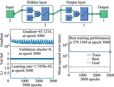
Fig.3.Architecture of the designed ANN and training state for P1.

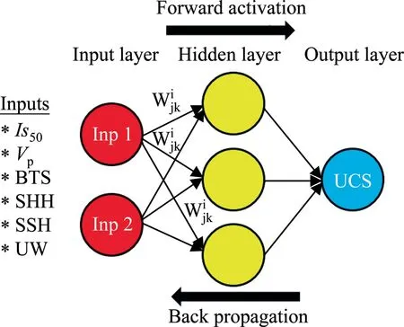
Fig.4.General ANN network structure employed in this study.

Table 5 shows the GEP parameters used for the training of all models.While creating the models,it has been ensured that it has a simple formulation and is practically usable.All multiple regression equations derived from GeneXproTools 5.0 program are given in Table 6.

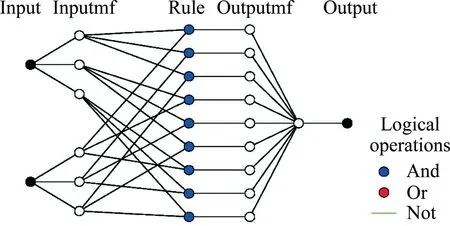
Fig.5.The structure of the constructed ANFIS in all models for the prediction of UCS.

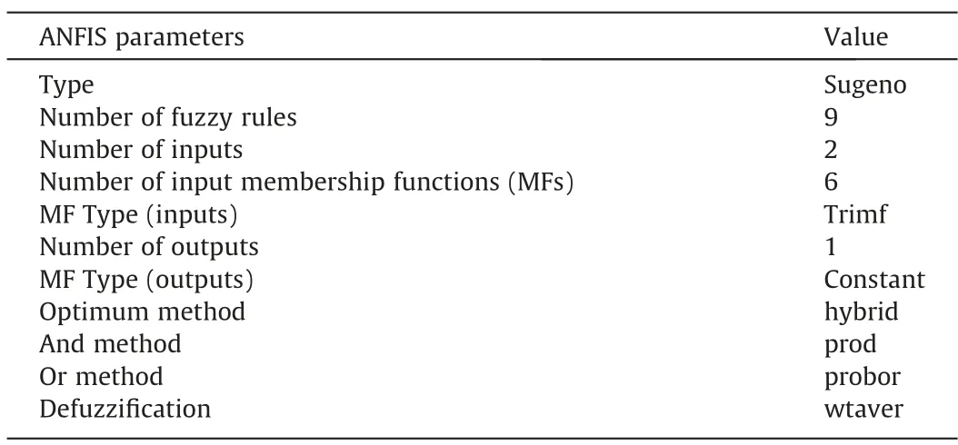
Table 4General properties of the ANFIS models.

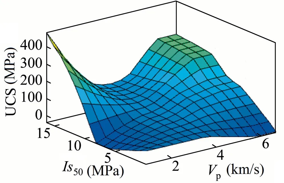
Fig.6.Surface graph demonstrating the association of UCS with Is50 and Vp (P1).

The fitness factor and R2versus generation iteration graphs obtained from the training dataset of Eq.(10) are shown in Fig.8.

Fig.7.Expression tree for Eq.(10).

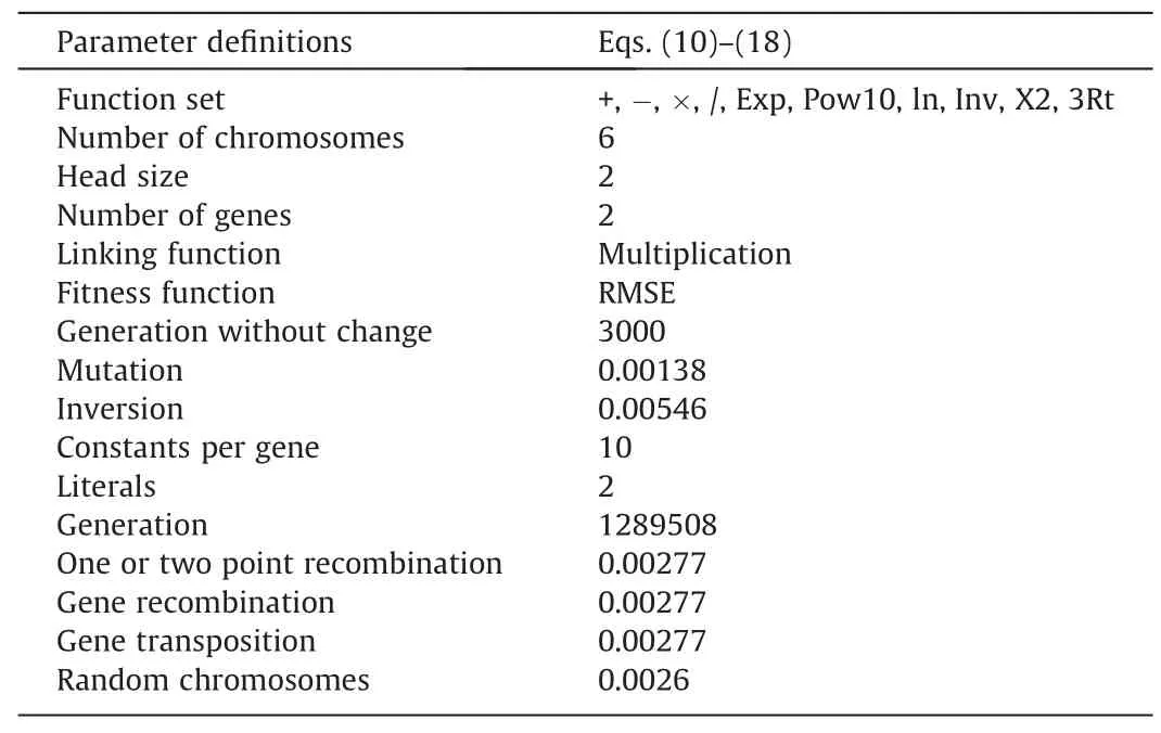
Table 5Parameters employed in the GEP models.

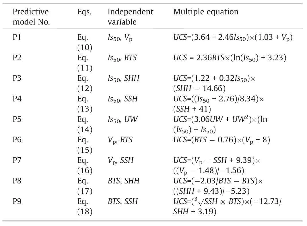
Table 6Equations obtained from the GEP (training dataset).

4.Results of models performances and comparison of models

4.1.Performance index

Fig.8.Fitness factor and R2 versus generation iteration (training dataset for Eq.(10)).

In order to check the estimation capacities of the derived models,some statistical performance indices (coefficient of efficiency,E; the root mean square error to observation’s standard deviation ratio,RSR; weighted mean absolute percentage error,WMAPE;the variance accounted for,VAF; adjusted determination coefficient,Adj.R2; and maximum determination coefficient,R2) were calculated for each model according to the Eqs.(19)–(24) given below.For all randomly selected datasets(training,testing,validating and full dataset) model performance indices were calculated.

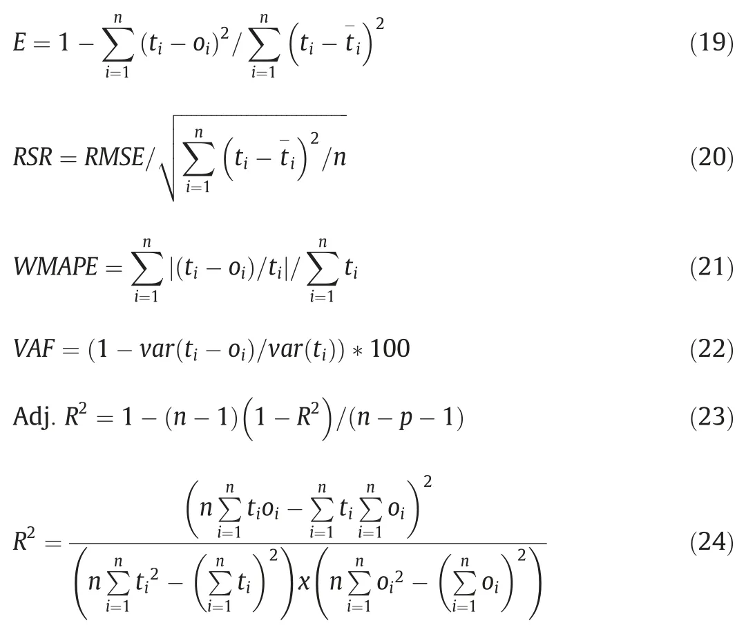
where t is the target UCS value obtained from the laboratory studies;o the output UCS value of models; ti the arithmetic mean of target UCS variables obtained from the formulas;the arithmetic mean of model variables;n the number of experimental study data;p the model input quantity; and var the variance:var （ti）=varience in set（ti）=

In addition,three of the model selection criteria(Hannan-Quinn information criterion,HQC; Bayesian information criterion,BIC;and Akaike’s information criterion,AIC) commonly used in MRA contexts,were calculated separately and the average of these three parameters was used as a new evaluation criterion.AIC is based on information theory using the Kullback-Leibler divergence for measuring the distance between the candidate model and the true model,whereas the BIC is based on Bayes’ factors.For these two parameters,which have different philosophies and approaches,the criterion in a regression context is very similar to one another,and the only difference is the right part(penalty)of Eqs.(25)–(27).In general,the smaller the AIC,BIC,and HQC values,the better the suitability.When comparing the models,it is preferred to have lower AIC,BIC,and HQC values.

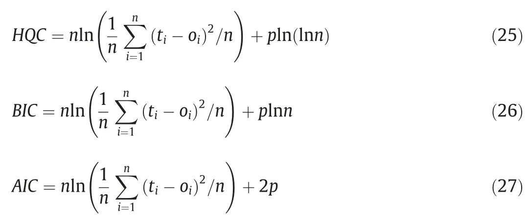
And as for performance index value,PIat,and the mean information criterion value developed by the author covered by this study,ICat,the following equations can be used.

Table 7PIat values of the developed models according to different techniques and datasets.

Table 8Comparison of all developed models according to PIat,ICat and Adj.R2.

where VAF is the variance account factor; WMAPE the weighted mean absolute percentage error of the prediction; Adj.R2the adjusted determination coefficient; E the coefficient of efficiency;and RSR incorporates the benefits of error index statistics and includes a scaling/normalization factor [57].

It is rather difficult to choose the most accurate model for the estimation of independent variables.Essentially,the accuracy of models can be examined separately using performance indices such as WMAPE,VAF,RMSE,RSR,and R2,but one of these indices is not superior to the others.Five of these performance indices were combined in the same formula and the performance index given in Eq.(28) was calculated to compare the performance of the developed models.Theoretically,for a model to be considered excellent,the Adj.R2and E values must be‘‘1′′,the VAF value‘‘100”,the WMAPE value ‘‘0” and the RSR value must be ‘‘0”.In this case,the theoretical PIatvalue of perfect estimation models should be equal to 3.Thus,the model with the highest PIatvalue is the most accurate and reliable one.The most reliable and accurate equations according to the PIatvalues are given in Table 7.

Table 7 shows the calculated PIatdata for all models of GEP,ANN,MRA,and ANFIS.In principle,values of full (training+test ing),training,testing,and validating datasets were summed.The arithmetic mean of the total values of these four different methods was compared (see Table 8).According to this criterion,the most reliable models are P2,P8 and P9,respectively.P3,P4 and P7 have lower performances than others.

The data of PIatin Table 8 were taken into consideration for the selection of the best performing method among the four different methods (GEP,ANN,MRA,and ANFIS) used in this study.When it is evaluated according to the sum of arithmetic means calculated for nine equations,it is seen that the MRA method which has the highest total value according to PIat(81.89) and lowest total value according to ICat(15,015) has the most successful performance.

The data of ICatin Table 8 was prepared using averages of AIC,BIC,and HQC values with similar principles in forming the data of PIatin Table 8.When the analysis of ICatpresented in Table 8 is evaluated,it is seen that the results obtained from PIatin Table 8 are confirmed.

In the presented models,relatively lower estimation errors were obtained in the test step compared to the training step.Test datasets satisfactorily reflect the generalization ability of the models.This is an indication that the learning process of predictive models is successful.

4.2.Anova

The estimation values obtained from MRA and whether the measured values have normal distribution were examined.Five statistical parameters are taken into consideration when deciding the normal distribution.These include the histogram graph,coefficient of variation,Kurtosis-Skewness,detrended Q-Q plots,and Kolmogorov-Smirnov normality test.As a result of evaluating a total of ten parameters,one of which is the measured UCS value,it is observed that most of the equations have a normal distribution and very few have abnormal distribution.After the normal distribution analysis,the dataset was analyzed using parametric and non-parametric methods.

4.2.1.Assuming the normal distribution of data

According to one-way analysis of variance,the predicted and measured variations were homogeneous (Levene statistic significance levels are 0.994,1.000,0.977,and 1.000,respectively,for GEP,ANN,MRA,and ANFIS).For the homogeneity of variance to be considered perfect,the significance level must be 1.000.According to the ANOVA results,there is no difference between the mean values of all groups (F statistical significance level is 1.000 for all models).Dunnett two-sided T test(post-hoc)was used for comparison of multiple tests to investigate the relationships between the measured and estimated values,where the measured values were taken as the control group (J group) for each main rock properties(Table 9 and Fig.9).The significance value to be used in the post hoc tests should be revised according to the total number of compared groups.The new significance value can be calculated using the following equation:NSV=0.05/[n(n-1)/2],where NSV is the new sig.value,0.05 is the 95% confidence interval value,and n is the number of groups.This value is calculated as 0.0011 for all properties.

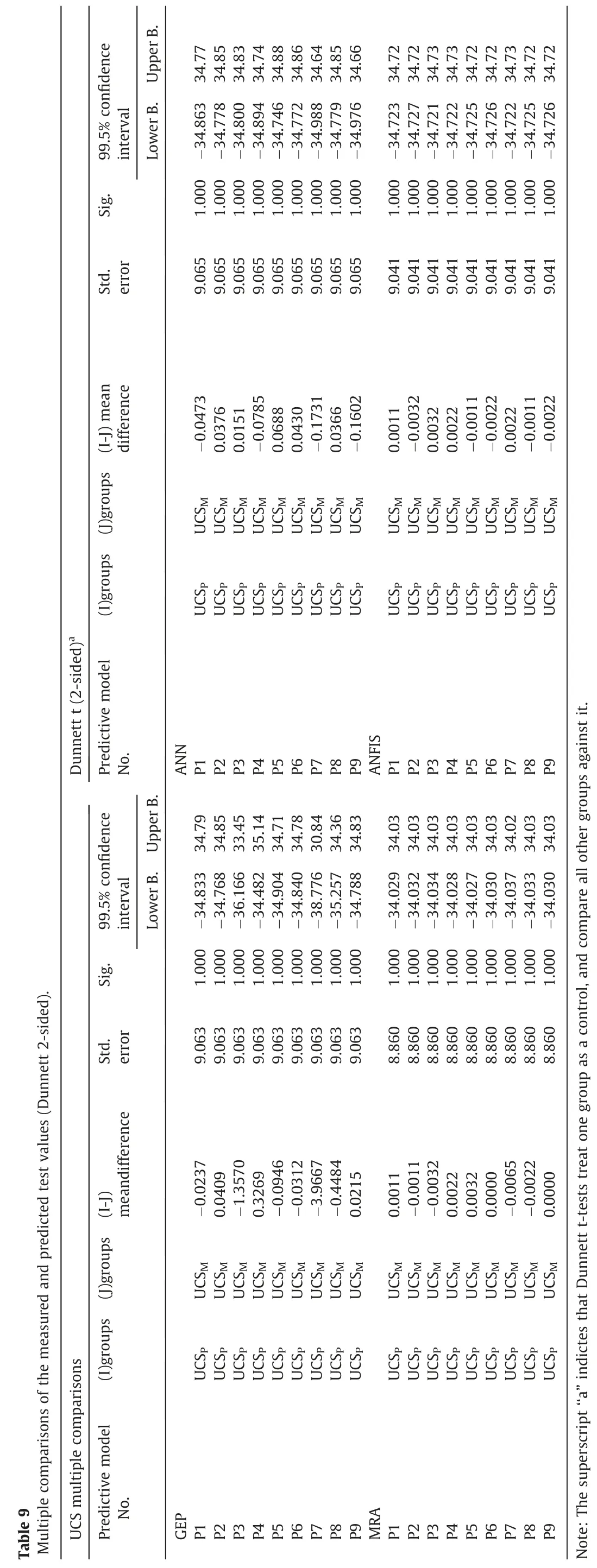
According to the Dunnett test,all data pairs have an equal standard error,very close mean difference,and an equal level of significance.In this case,given the results of the ANOVA analysis and the correlation,any derived equation can be safely used to estimate the UCS of the rocks.

4.2.2.Assuming the abnormal distribution of data

The Welch ANOVA method was used for the nonparametric test.Tamhane’s T2 test(post-hoc)was used for comparison of multiple tests to investigate the relationships between the estimated and measured values.Variations of the measured and predicted values were found to be homogeneous by Welch ANOVA analysis(Welch statistic significance level is 1.000 for all models).According to Tamhane’s T2 test (post-hoc) test results,it can be said that there is no significant difference between the groups because of the remarkable values (equal to 1 for all equations) > 0.05,i.e.the groups were homogeneously distributed.

4.3.Graphs

The results of the constructed different equations were plotted on a scatterplot showing the target(measured)versus model(predicted).One of the ways to find the estimation capacities of the models is to draw the data points of the measured and predicted output according to the line y:x (1:1).The point that lies on the y:x line shows the exact prediction of the output by the model and closer a point to the y:x line,the better is the prediction.These scatterplots were plotted for full,training,testing,and validating datasets of the nine equations and graphs plotted for training,testing,and validating datasets in Fig.10 were given separately for the GEP,MRA,ANN,and ANFIS programs.The plotted points were lying close to the y:x line,implying a successful prediction of all models.

In this section of the study,the performance of the models obtained from the programs used in the data analysis was compared.After the training,the models were tested with a dataset consisting of 28 test samples.All models ensured satisfying results in terms of statistical performance criteria for prediction of UCS.These models designed to cover all rock types are considered to be valid for the prediction of the UCS.Regression plots for the full,training,testing and validating data set of the models with the strongest (P2) and the weakest (P7) performance among the produced nine equations are shown in Fig.11.The high correlation coefficients seen in Fig.11 show how successful the derived models are in predicting the output.

Scatter plots(Fig.12)of UCSMand UCSPvalues are plotted to see the predictability of the best multiple models (P2 and P9 by using the GEP,ANN,MRA,and ANFIS,respectively).The scatter plots contain the maximum and minimum confidence interval lines as well as the maximum and minimum prediction lines calculated for the 95% confidence interval.When Fig.12 is examined in detail,it is seen that only one or two rocks out of 93 rocks are outside the limits of estimation (for all estimation tools).

Fig.13 shows the distribution of UCSMand UCSPvalues and residuals by data number according to the program type.Considering the residuals of the models,we can see that the most stable result for P2 is the MRA program.In ANN,ANFIS and GEP graphs,it is seen that residuals change in larger value range especially in validating dataset.

Fig.9.Comparison of the mean values of the UCS tests obtained from different methods.

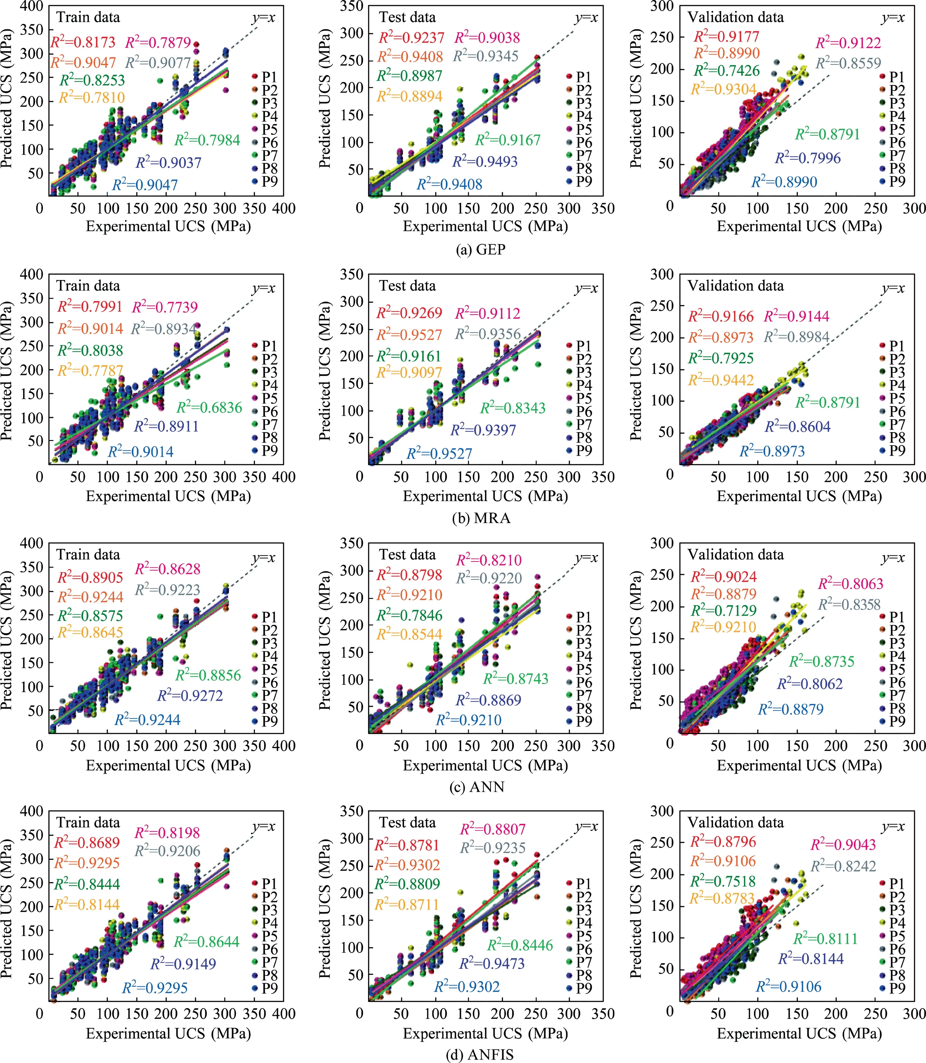
Fig.10.R2 of predicted and measured values of UCS for training,testing,and validating datasets.

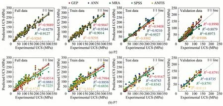
Fig.11.Comparison of experimental and predicted UCS values according to program type (the best P2,the worst P7).

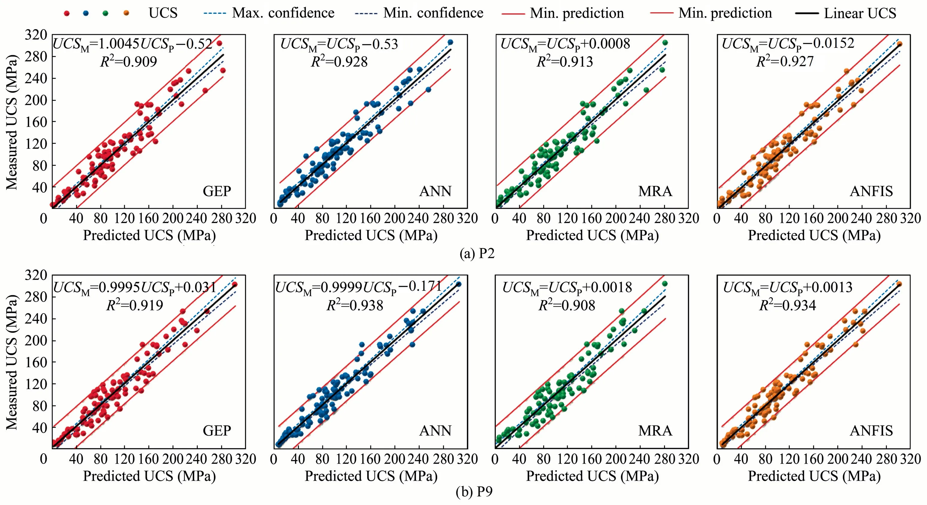
Fig.12.Comparison of measured and predicted UCS values of the determined best model according to different methods (P2 and P9).

5.Results and summary

In this research,several modeling techniques (SRA,MRA,ANN,ANFIS,and GEP)have been utilized for predicting the UCS of rocks using some features including BTS,SHH,SSH,Is50,Vpand UW of rocks.In addition,models with high correlation coefficients that can be used in engineering applications were determined.The datasets were modeled with the help of these statistical programs and compared with each other to choose the best model.In addition,the UCS values obtained from the models were compared with the real UCS values obtained from the laboratory study with the help of various graphs and some statistical parameters.

Very high correlations were obtained between UCSMand UCSPfor all prediction tools at a 95% confidence level.According to the one-way analysis of variance,the variations of UCSMand UCSPvalues were found to be homogeneous.There was no difference between the average values of the UCS groups according to ANOVA.According to Dunnett’s two-sided T test,each data pair had an equal standard error,a very close mean difference,and a level of significance.According to the results of ANOVA analysis,all equations obtained with different estimation tools can be used safely in estimating UCS of rock samples.

As is known,the accuracy of the models can be examined separately using performance indices such as WMAPE,VAF,RMSE,RSR and R2,but one of these indices is not superior to the others.In literature,some performance indexes have been published to eliminate the difficulties encountered in determining the accuracy of the derived models.In this study,five of the performance indexes were combined in the same formula and thus a more accurate evaluation was aimed.In the developed new performance index,PIat=3 should be theoretically perfect for a model.The results of this study showed that the new index can be used safely by the researchers.

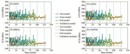
Fig.13.Distribution of UCSM and UCSP values and residuals with data number according to method type (P2).

If Adj.R2values are taken into consideration,it is seen that ANFIS and ANN methods give better values than GEP and MRA methods.This leads to the conclusion that it would be more accurate to use a more comprehensive evaluation index,such as the PIatvalue proposed in the article,rather than a single performance evaluation index when choosing from equations with very close performances.

6.Conclusions

According to the performance index assessment,the weakest model among the nine models is P7 (Vp-SSH),while the most successful models are P2 (BTS-Is50),P9 (BTS-SSH),and P8 (BTS-SHH),respectively.

When the models developed for UCS with the highest performance estimation are examined,it is seen that one of the two independent variables is the BTS test.BTS is one of the basic rock parameters and the result is not surprising since it is controlled by the same factors as UCS.

The PIatand ICatperformance indices developed by the author were used to select the best performing method among the four different prediction tools (GEP,ANN,MRA,and ANFIS).Among these four methods,which are found to have very close performance values,the MRA method is the most successful method with very small difference.

When the validating dataset,which has been collected from different studies in literature,is added to the performance evaluation,it is seen that the MRA method,which has more stable results,is the most successful.The ANN and ANFIS methods,which obtained very successful results with training and testing data obtained from 93 rock samples,is the most unsuccessful when the validating dataset is included.In fact,while the superiority of ANFIS and ANN decreases as the linearity and dimensionality of the problem decreases,traditional regression techniques often make the right approaches in such a situation.

Another finding in the performance evaluation is that the testing dataset is the most successful group and the validating dataset is the most unsuccessful group.The reason for the poor performance of the validating dataset is obvious.For example,the validating dataset of P3 is formed with data collected from 21 different articles.This shows that the same test was carried out by 21 different researchers using test instruments with different calibration properties.In spite of this handicap,the results obtained with the validating dataset successfully demonstrate the accuracy of the equations obtained from the study.