BIFURCATION ANALYSIS OF A CLASS OF PLANAR PIECEWISE SMOOTH LINEAR-QUADRATIC SYSTEM∗†

Qiwen Xiu,Dingheng Pi

(Fujian Province University Key Laboratory of Computational Science,School of Mathematical Sciences,Huaqiao University,Quanzhou 362021,Fujian,PR China)

Abstract

Keywords piecewise smooth systems;limit cycle;sliding cycle;pseudohomoclinic bifurcation;critical crossing bifurcation CC

1 Introduction

The bifurcation theory of planar smooth differential systems has developed very fast since D.Hilbert put up the famous Hilbert’s 16th problem(see e.g.[19]and[23]).In recent years,piecewise smooth(PWS for short)dynamical systems with some parameters have been widely applied in many fields,such as mechanics,electronics,control theory,biology,economy and so on.They are also used to explain some phenomena such as pest control or model some mechanical systems exhibiting dry friction and electrical circuits having switches and so on.These wide applications and study of Hilbert’s 16th problem are important sources of motivation of bifurcation analysis in PWS systems(see e.g.[7,16,20,30-32]).

Filippov established some systematic methods to study qualitative theory of PWS systems in his book[9].Kuznetsov et al.studied one-parameter bifurcations in planar Filippov systems.They gave an overview of all codimension one bifurcations including some novel bifurcation phenomena that can only appear in planar PWS systems in[21].Guardia et al.studied local and global bifurcation in PWS systems in[14].Many novel bifurcation phenomena that will not be seen in smooth systems have been hot issues of bifurcation problems of PWS systems such as sliding bifurcation,critical crossing cycle bifurcation and so on.Freire et al.studied critical crossing cycle bifurcation and pointed out that critical crossing cycle bifurcationCCcan occur in co-dimension one bifurcation,but critical crossing cycle bifurcationCC2cannot occur in co-dimension one bifurcation problems(see[12]).

When subsystems of planar PWS systems have the same type of singularities and different types of singularities,their bifurcation problems have been widely studied in the past few years.Even for planar PWS linear systems defined in two zones,their bifurcation problems are not easy to be studied.People have found many novel bifurcation phenomena that will not appear in smooth linear systems(see[13,15]).It is not easy for people to discuss bifurcation phenomena of planar piecewise linear systems with many parameters.Luckily,Freire et al.gave a Linard-like canonical form for a class of piecewise linear systems with two zones.When each subsystem has no equilibrium point in its own zone and if each subsystem has a focus,they showed that two limit cycles can exist(see e.g.[10]).PWS linear systems with node-node dynamics and saddle-saddle types were considered in[17]and[18],respectively.

Recently,bifurcation phenomena of planar PWS systems that are constituted by linear system and quadratic Hamiltonian system have been studied by some authors(see e.g.[22,27-29]).

Li and Huang[22]considered the following PWS system

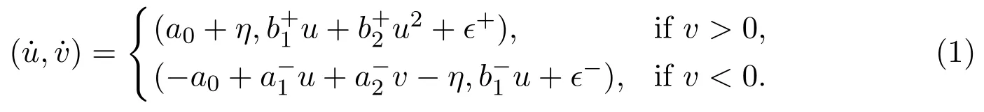
Under their assumptions,the linear system has a saddle.They got the following system which is topologically equivalent to system(1)

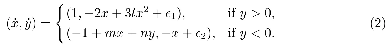
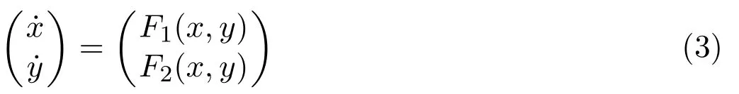
The unperturbed system of(2)is the following system(3).See equation(7)in[22].

This PWS system is made up of a quadratic Hamiltonian system and a linear system

with

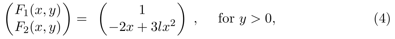
and

wherel(0),m,nare 3 real parameters.

When the subsystem of PWS systems has a fold,many bifurcation phenomena will occur.PWS systems with 3 parameters were discussed by Buzzi et al.in[4].They discussed a special unfolding for PWS systems having a fold-cusp singularity.System(4)also has some folds(that is tangency points of second order).The definition of fold and cusp can be found in[14](see Definition 2.1).

Li and Huang[22]assumed that these parameters satisfy some conditions,then the linear system has a saddle and its quadratic system has some folds.They discussed the homoclinic bifurcation of system(3).Moreover,they discussed Hopf bifurcation for a perturbed system of system(3).For more general scenarios,the stability and perturbations of generalized loops of planar PWS systems have been studied by applying Melnikov function.The loop has a saddle and a tangency point(see Figure 1 of[5]).Limit cycles bifurcating from generalized homoclinic loops having a tangent points were studied by analyzing Poincarmap and the authors found at most two limit cycles can appear in the related planar PWS systems(see[24]).Under the assumption that there exists a family of periodic orbits on the inner(resp.,outer)side of the homoclinic loop,Liang and his collaborators studied homoclinic bifurcations of planar PWS systems with a generalized homoclinic loop having a saddle-fold point by analyzing the asymptotic expansion of the first order Melnikov function corresponding to the period annulus in[25].

As the parameters vary,the linear system of(1)will have a focus or a node.We can still have similar form as given by system(2).To our knowledge,when one subsystem has a fold and the other subsystem has a focus or a node,we still know little on their bifurcation phenomena.However,Li did not consider these scenarios in[22].A natural question is:Does system(2)have other bifurcation phenomena when its linear subsystem has a node or a focus?This problem deserves to be further studied.Indeed,we find some interesting bifurcation phenomena in this paper.

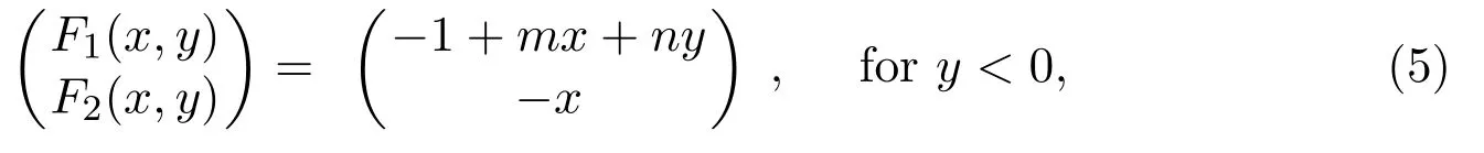
In this paper we shall first investigate bifurcation phenomena of the unperturbed system(3).In the sequel,we study bifurcation phenomena of system(2).At this moment,the linear system(5)has a focus or a node.Let Σ ={(x,0)|x∈R}.In what follows we call equation(3)with(4)the upper system of(3)and equation(3)with(5)the lower system of(3).We denote upper system and lower system of(3)byf+(x,y)andf−(x,y),respectively.Our results will show that when the linear system(5)has a focus or a node,system(3)has a sliding cycle and undergoes pseudo-homoclinic bifurcation and critical crossing bifurcationCC.These novel bifurcation phenomena will not appear in smooth planar differential systems.

From[21](see P2171),we know that one can construct a local transversal section to a stable sliding cycle and define Poincarmap in the usual way forward in time.Note that all nearby points will be mapped into the fixed point of Poincarmap,the derivative of Poincarmap at the fixed point corresponding to the sliding cycle will be zero.This is referred to as superstability.In this case Poincarmap is not invertible.However,a generic crossing cycle has a smooth invertible Poincarmap.We often use the derivative of Poincarmap to discuss the stability of a crossing cycle.If the derivativeµof Poincarmap satisfiesµ<1,the crossing cycle is exponentially stable.If the derivativeµof Poincarmap satisfiesµ>1,the crossing cycle is exponentially unstable.A crossing critical cycle is a crossing cycle passing through the boundary of a sliding segment.The crossing critical cycle is the intermediate situation between a sliding cycle and a crossing cycle.

We recall definitions of critical crossing cycle bifurcationsCCandCC2for the sake of completeness(see[12]and[21]).When planar PWS systems with parameterαundergo critical crossing bifurcationCC,there is a sliding cycle with a single sliding segment ending at a tangency point when the parameterα<0.This sliding segment shrinks forα→0.The sliding cycle becomes a crossing critical cycle whenα=0.Then the critical crossing cycle disappears forα>0 forming an exponentially stable crossing limit cycle.SeeCCof Figure 17 in[21].

When planar PWS systems with the parameterαundergocritical crossing bifurcation CC2,a superstable sliding cycle coexists with an exponentially unstable crossing cycle for sufficiently small parameterα<0.The two cycles collide atα=0 forming a critical crossing cycle and then disappear forα>0.This bifurcation implies the catastrophic disappearance of a stable sliding cycle.

This paper is organized as follows.In Section 2 we will state our main results.Their proofs will be given in Section 3.Some examples will be given to apply our results in Section 4.We give our conclusions in Section 5.

2 Statement of the Main Results

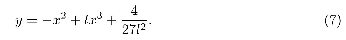
Before we state our main results,we need some basic facts on the upper and lower systems of(3).The orbits of upper system(4)are some cubic curves

The upper half system of(3)has two folds on Σ,that is,the originO(0,0)and point.Moreover,the pointBis visible and the pointOis invisible.Its orbit passing through the pointBwill have another intersection point with Σ,denoted by.We substitute the coordinates of the pointBinto equation(6),we get that.So the expression of the orbit that goes through the pointBis

If system(3)has a closed cycle(except sliding closed cycle),it must intersect Σ and is located betweenBand.The following lemma will be used in the proof of our main results(see[9]).

Lemma 1Consider the equation

where G is of class C4at the origin satisfying

for(x,y)near the origin.Let y=Y(x)be the solution of(10)satisfying

then for small enough r>0

where

Proposition 10,then the following statements hold.

(1)Define P+(0)=0,then P+is continuous at the point x0=0.In addition,the first four derivatives of P+at the point x0=0are

(2)P+is decreasing with respect to x0,and concave from below(above)if l<0(l>0).

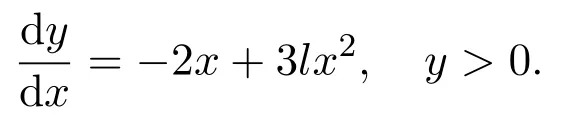
Proof(1)The upper system(4)can be rewritten as the

We get from Lemma 1 that

for small enough−x0>0,where

By equation(12),we have

Moreover,we obtain first four derivatives ofP+at the pointx0=0.Thus the statement(1)of Proposition 1 follows.

(2)We only need to prove the statement whenl<0.Whenl>0,the statement can be proved similarly.By(9),ifl<0,we have

It is clear thatx11>0 andx12<0 whenl<0.Since,x12should be discarded.The useful root ofh(x1)=0 is

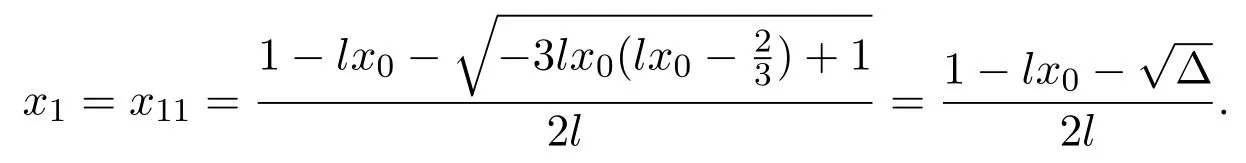
Sincex1=P+(x0),we have

Since 3lx0−1<1 andfor all,we know thatandP+(x0)is decreasing with respect tox0.

Easy calculation shows that

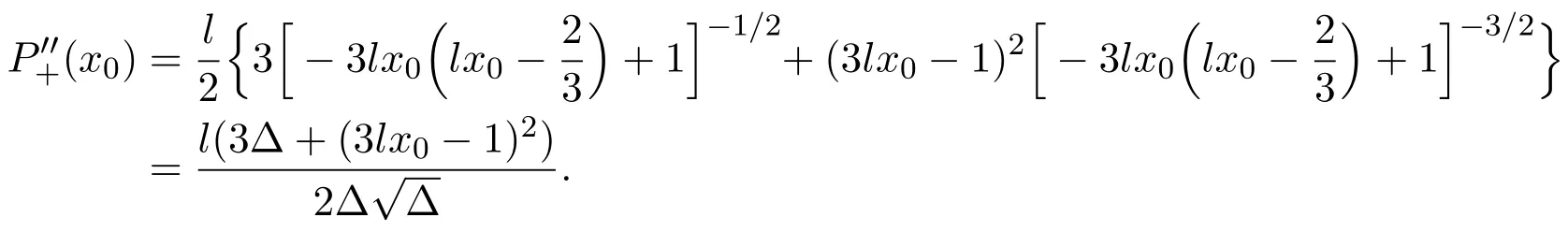
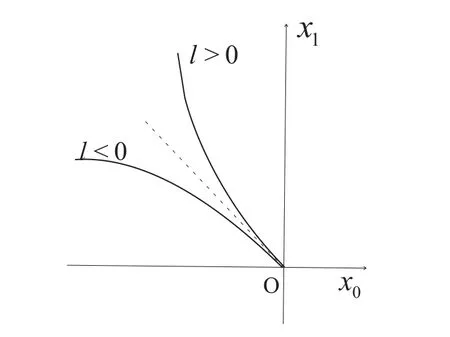
Figure 1:Graphs of the Poincar map P+with different l

System(5)has a unique singularity.In what follows we will discuss the scenarios whenSis a focus of the lower linear system and thenSis a node of the linear system.For each scenario,we will provide a bifurcation analysis for the planar PWS system.

2.1 The lower system with focus dynamic

In this case,the singularityof lower system is a focus.We need the assumption.Let,the eigenvalues ofare the following

The solution of the lower system with initial value(x0,0)att=0 is

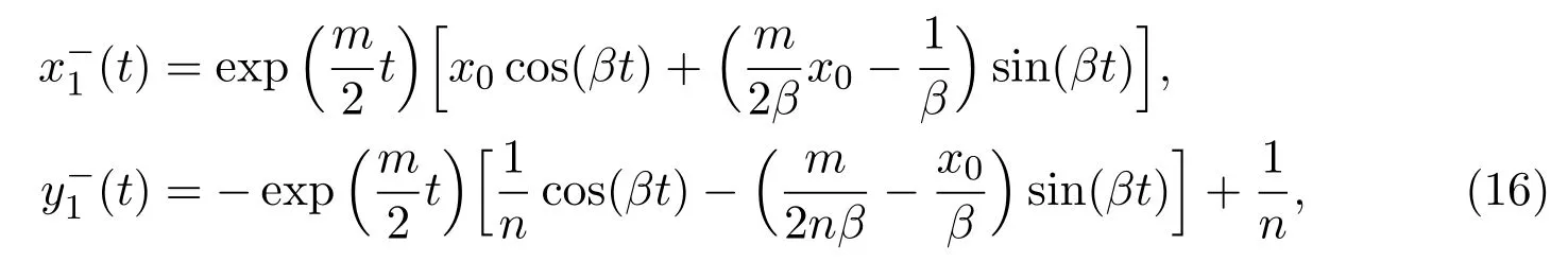
wheret>0.The orbits of lower system surrounding originOrotate clockwise.Then the orbit of lower system starting at(x0,0)withx0>0,will arrive at Σ at the point(x1,0)withx1<0 after a certain timet1>0.We define a lower PoincarmapP−asx1=P−(x0)withP−(0)=0.Then we have

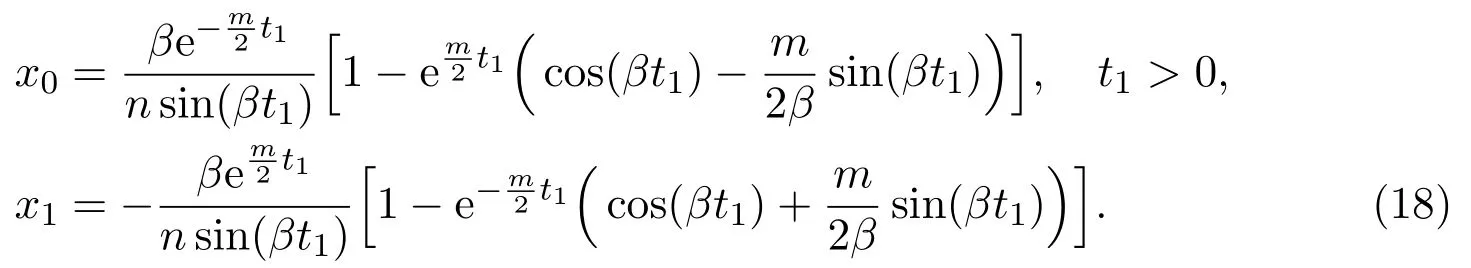
Here,we ask thet1>0 to be minimum time such that(17)holds.Since the singularitySis not in the lower half plane,βt1∈(0,π).It means that sinβt1>0 forβt1∈(0,π).Therefore,we obtain the parametric representations of lower PoincarmapP−from equations(16)and(17)

For brevity,sets=βt1and,the above two equations can be written as

wheres∈(0,π),φmγ(s)=1−emγs(coss−mγsins).This function has been introduced in[1]and[10].It has the following symmetry properties

Figure 2 gives the graph ofφmγ(s).For the lower PoincarmapP−,we have the following proposition.

Figure 2:The graph of φmγ(·)for a positive value of m

Proposition 2Suppose that system(5)satisfies the assumption,m∈R,s=βt1and,then the following statements hold.

(1)x0is increasing with respect to s and x1is decreasing with respect to s,with

(2)When m=0,P−(x0)=−x0for all x0>0.

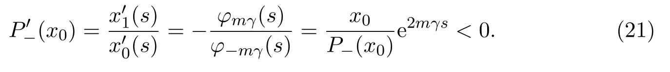
(3)0,for all x0>0,we have P−′(x0)<0and

ProofIt follows from(19)that

Figure 2 and the symmetry properties ofφmγ(s)imply thatφmγ(s)andφ−mγ(s)are always positive whens∈( 0,π).Using the factn>0,β>0,,we havefors∈( 0,π).Moreover,easy calculation shows that

We get from(20)that

Whenm=0,.By(21),P−(x0)=−x0,for allx0>0.When0,it is clear thatfor allx0>0.P−is decreasing with respect tox0.Furthermore,

From(21),we have

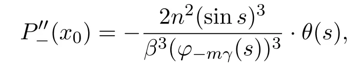
whereθ(s)=sinhmγs−mγsins.We get from signθ(s)=signmthat sign.The proof is complete.

2.2 Sliding dynamics

In this part,we shall discuss the sliding dynamics of PWS system(3).Whenl<0,system(3)has an attracting sliding region.Whenl>0,system(3)has a repulsive sliding region.LetM(x,0)∈Σ,then the vector fields of upper and lower systems at pointMare as follows

and

In fact,since the points in the sliding region must satisfy

It follows that the sliding regionsare aforementioned.Now we establish the sliding vector field onby Filippov convex method.The sliding vector field

should be tangent to Σ,it follows that

In the following proposition,we will find that the sliding vector fieldYsmay have a pseudo-saddle.The definition of pseudo-saddle was given in Definition 2.8 of[14].

Proposition 3For the sliding vector field Yswith l<0,m>0,there exists aunique singularitywhich is a pseudo-saddle.

ProofSetg(x)=3lmx2−(3l+2m)x+3.Whenl<0 andm>0,the root of discriminant ofg(x)satisfies∆=(3l+2m)2−36lm>0.Two roots ofg(x)=0 are the following

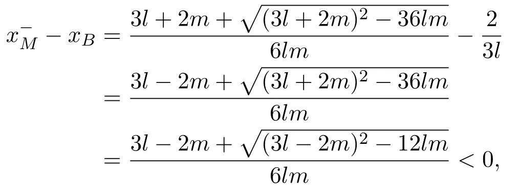
wherexBis the abscissa of pointB.Since 3lx−1>0 for allis always on the left of pointB.Moreover,Yshas a unique singularityin the regionwhenl<0,m>0.M−is a pseudo-saddle.The proof is complete.

Analogously,we have the following results whenl>0 andm<0.

Proposition 4For the sliding vector field Yswith l>0and m<0,there existsa unique singularity,which is a pseudo-saddle.

In what follows we present two main results when the lower linear system has a focus.

Theorem 1Suppose that system(3)satisfies the basic assumptionandl<0.Then the following statements hold.

(1)If m≤0,system(3)has no periodic orbit.

(2)If m>0and,there exist l1,l2satisfyingsuchthat the following statements hold.

(a)If,system(3)has a stable limit cycle(crossing periodic orbit).

(b)If l=l1,system(3)has a stable crossing critical cycle.

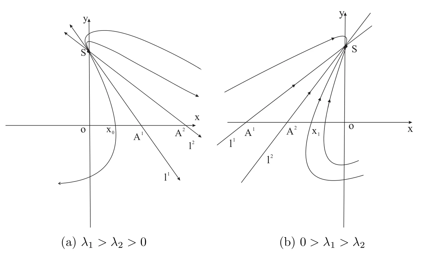
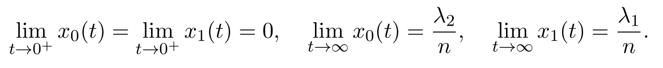
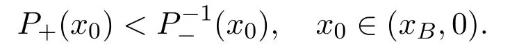
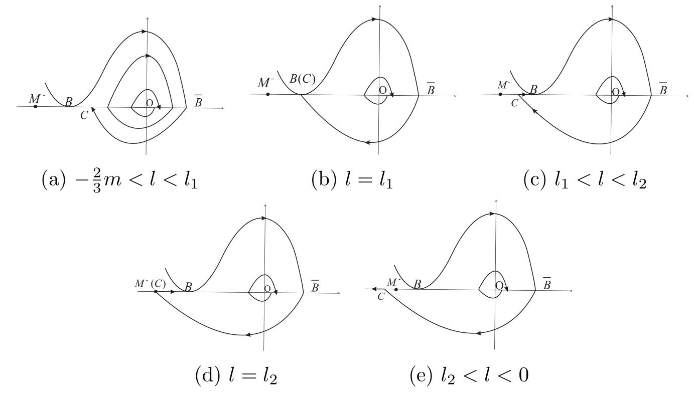
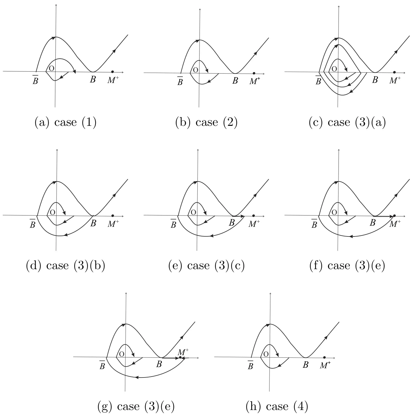
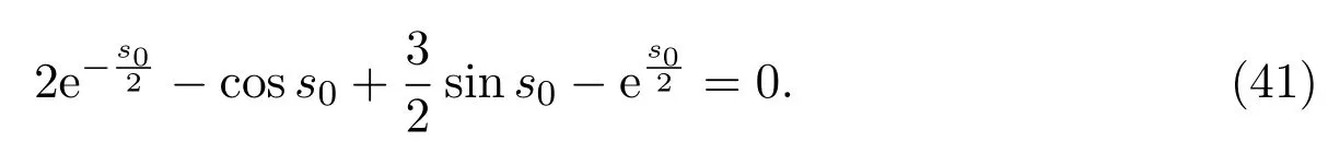
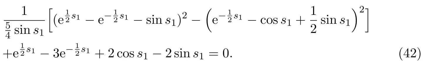
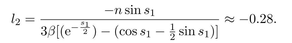
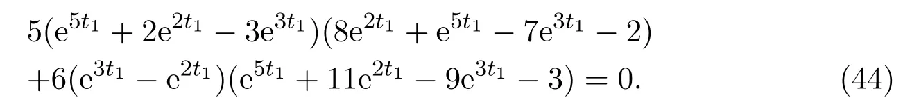
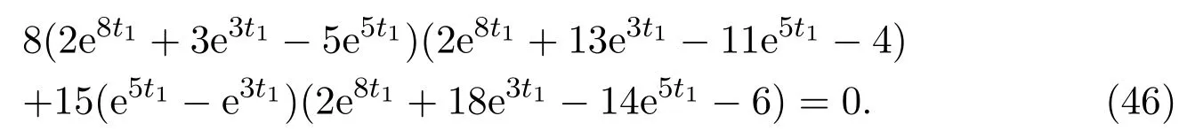
(c)If l1

(d)If l=l2,system(3)has a sliding homoclinic cycle,which is stable.

(e)If l2

(3)If m>0andthere are no corresponding l1,l2that satisfySo system(3)has no periodic orbit.

Theorem 2Suppose that system(3)satisfies the basic assumptionandl>0.Then the following statements hold.

(1)If m≥0,system(3)has no periodic orbit.

(2)If m<0andthen there exist l1,l2satisfyingsuch that the following statements hold.

(a)If,system(3)has an unstable limit cycle(crossing periodicorbit).

(b)If l=l1,system(3)has an unstable crossing critical cycle.

(c)If l1>l>l2,system(3)has an unstable sliding cycle.

(d)If l=l2,system(3)has a sliding homoclinic cycle,which is unstable.

(e)If0

(3)If m<0and,then there are no corresponding l1,l2that satisfy.So system(3)has no periodic orbit.

2.3 The lower linear system with node dynamics

In this section,we assume thatm2>4n>0.Sis a node of the lower linear system.Direct computation shows that

whereλ1,λ2are the eigenvalues ofand Ψλ1,λ2(t)=λ1− λ2+λ2eλ1t−λ1eλ2t.Letl1andl2be the invariant manifolds of lower system,then we have

l1andl2intersect Σ at points,respectively.

Proposition 5Suppose that system(5)satisfies the assumption m2>4n>0and λ1>λ2,then the following statements hold.

(1)x0(t)is increasing with respect to t and x1(t)is decreasing with respect to t.

(2)When λ1>λ2>0(that is,m>0),P−given in(24)is defined onand

(a)P−is decreasing and convex with respect to x0.

(b)P−hasas an asymptote.

(3)When0>λ1>λ2(that is,m<0),P−is defined on(0,+∞)and

(a)P−is decreasing and concave with respect to x0.

(b)P−hasas an asymptote.

(4)Define P−(0)=0,then P−is continuous at the point x0=0.In additiontothis,the first four derivatives of the P−at the point x0=0are

Graphs ofP−for differentmare shown in Figure 3.

Figure 3:Graphs of the lower Poincar map P− for different m

Proof(1)We get from(24)that fort>0

Sincen>0,λ1λ2>0,λ1>λ2,we have Ψλ1,λ2(t)>0, Ψλ1,λ2(−t)>0.ThenThis implies thatx0(t)is increasing with respect totandx1(t)is decreasing with respect tot.

(2)Whenλ1>λ2>0,we obtain

Moreover,by(25)we have

ThusP−is decreasing with respect tox0with a domain given byand hasas an asymptote.Direct calculation from(25)gives

(3)When 0>λ1>λ2,by(24),we know that

Thus,the domain ofP−is(0,+∞)and the asymptote is.Sincem<0,similarly we haveis decreasing and concave with respect tox0.

(4)According to the analysis given in proving statement(2),the continuity ofP−at the pointx0=0 is obvious.Using an approach similar to that in[18],we obtain Finally we have the first four derivatives ofP−at this point.0>λ1>λ2,respectively.The domain ofP−isand the range of

Figure 4 shows phase portraits of the lower system of(3)whenλ1>λ2>0 andP−iswhenλ1>λ2>0(0>λ1>λ2).

Theorem 3Suppose that system(3)satisfies m2>4n>0and l<0.Thenthe following statements hold.

(1)If m<0,system(3)has no periodic orbit.

(2)If m>0(that is,λ1>λ2>0),,system(3)has no periodic orbit.

(3)If m>0(that is,λ1>λ2>0),there exist l1,l2satisfyingsuch that the following statements hold.

(a)If−23m

(b)If l=l1,system(3)has a stable crossing critical cycle.

Figure 4:Phase portraits of lower system of(3)

(c)If l1

(d)If l=l2,system(3)has a sliding homoclinic cycle,which is stable.

(e)If,system(3)has no periodic orbit.

(4)If m>0(that is,λ1>λ2>0),,there are no corresponding l1,l2that satisfy.So system(3)has no periodic orbit.

Theorem 4Suppose that system(3)satisfies m2>4n>0,l>0.Then the following statements hold.

(1)If m>0,system(3)has no periodic orbit.

(2)If m<0(that is,0>λ1>λ2),,system(3)has no periodic orbit.

(3)If m<0(that is,0>λ1>λ2),,then there exist l1,l2satisfyingsuch that the following statements hold:

(a)If,system(3)has an unstable limit cycle(crossing periodicorbit).

(b)If l=l1,system(3)has an unstable crossing critical cycle.

(c)If l2

(d)If l=l2,system(3)has a sliding homoclinic cycle,which is unstable.

(e)If,system(3)has no periodic orbit.

(4)If m<0(that is,0>λ1>λ2),,then there are no correspondingl1,l2that satisfy.So system(3)has no periodic orbit.

2.4 Hopf bifurcation

From[6,15,22]we know planar piecewise smooth system will undergo Hopf bifurcation near singular points of focus-focus(F-F)type,focus-parabolic(F-P)type,parabolic-parabolic(P-P)type.When the linear system has a focus,the origin of system(1)is a pseudo-focus of P-P type.We have the following results.

Theorem 5Assume that,l<0,the following statements hold.

(i)Ifandhold,then for0<ϵ2≪1,the P-P focus Pϵof system(2)is asymptotically stable.

(ii)If,the origin of system(3)is an asymptotically stable pseudo-focusof order4.

(iii)Ifhold,then for0<ϵ2≪1,the P-P focusPϵof system(2)is unstable.Moreover,system(2)has a stable limit cycle and anunstable limit cycle if.

Theorem 6Assume thatand l>0,the following statements hold.

(i)Ifhold,then for0<−ϵ2≪1,the P-P focusPϵof system(2)is unstable.

(ii)If,the origin of system(3)is an unstable pseudo-focus of order4.

(iii)Ifhold,then for0<ϵ2≪1,the P-P focusPϵof system(2)is asymptotically stable.Moreover,system(2)has an unstable limitcycle and a stable limit cycle ifand0<−ϵ2≪1.

From the above two theorems,we find that Hopf Bifurcation and critical crossing bifurcation occur.Ifl>0,we shall have similar results.When the linear system has a node,the origin of system(1)is a pseudo-focus of P-P type.We have similar bifurcation phenomena.

3 Proof of the Main Results

In this section,we will prove our main results.

We recall some results in[22].The equilibrium point of linear system is a saddle.The eigenvalues ofare the followingλ1andλ2.Other notations in the following proposition have similar meanings with Proposition 5.

Proposition 6Suppose that system(5)satisfies the assumptions n<0,m∈Rand λ1>0>λ2,then the following statements hold.

(1)x0(t)is increasing with respect to t and x1(t)is decreasing with respect to t,

(2)P−is decreasing with respect to x0,P−is concave(convex)when m<0(m>0).

(3)When m=0,P−(x0)=−x0,where.

(4)Define P−(0)=0,then P−is continuous at the point x0=0.In addition to this,the first four derivatives of the P−at the point x0=0are

Remark 1Easy calculation shows that the process of obtainingP−(x0)has nothing to do with the sign ofnand the fact that whetherλ1,λ2are real roots or not,it follows thatP−(x0)still has the above expression in the case of focus.Moreover,direct calculation shows that the inverse ofP−(x0)has the following expression

The graph ofP−(x0)is similar to that of.

3.1 Proof of Theorem 1

(1)By Proposition 1,P+(x0)is convex and decreasing with respect tox0whenl<0.Since,P+(x0)<−x0for allx0∈(xB,0).By Proposition 2,forx0∈(−∞,0)whenm≤0.Then

(2)By Proposition 2,x0is increasing with respect tosfors∈( 0,π)

For a givenl<0,there exists a uniques0∈( 0,π)such that

System(3)has a critical crossing cycle which is equivalent to there exists ans0∈(0,π)such thatthat is 2x0(s0,m)+x1(s0,m)=0.Note thatlis unknown,we should determines0.By(19),we have

It follows that

Actually,in this cases0is independent ofl.We will give a graph to show that for suitable values ofk=mγ>0,indeed there exists ans0∈(0,π)such that equation(29)holds.With the help of computer,we know there exists ans0∈(0,π)such that the equation holds for suitable values ofk>0.See Figure 5.

Figure 5:The graph of the function in equation(29)

Set

Ifl=l1,thenthus system(3)exists a critical crossing cycle.

If there exists ans1∈(0,π)such thatand,then system(3)will have a sliding homoclinic cycle.Therefore,we need the following equations

We eliminatelfrom the above two equations and note thatl<0,we have the following equation

whereT=(emγs1−e−mγs1−2mγsins1)2−(e−mγs1−coss1+mγsins1)2.Analogously,s1is independent ofl.There are suitable valuesk=mγ>0,indeed there exists ans1such that equation(31)holds.Since it is not easy to solve equation(31),in what follows we will give another graph to show there exists ans1∈( 0,π)such that equation(31)holds.Letk=mγ>0,then we have the following equation

With the help of Matlab,we have Figure 6.It shows that there exists ans1∈(0,π)such that the equation holds for suitable values ofk>0.

Figure 6:The graph of the function in equation(31)

Set

Ifl=l2,thenthus system(3)exists a sliding homoclinic cycle.

From Proposition 1 and the above remark,we have

where−x0>0 is small enough.

This means thatCis always on the right ofB.Moreover,Using the monotonicity and concave properties ofP+,,there exists a uniquesuch that,and

Hence system(3)has a stable limit cycle(crossing periodic orbit),see Figure 7(a).

Ifl=l1,then This means thatCcoincides withB.System(3)has a stable crossing critical cycle,see Figure 7(b).

Ifl1

Ifl=l2,then

This means thatCcoincides withM−.The sliding homoclinic cycle is stable,see Figure 7(d).

Ifl2

Figure 7:The topological structures of trajectories in(3)of Theorem 1

(3)We prove this part by contradiction.If there arel1,l2that satisfy.That is,whenm>0,,the orbit of the lower system will coincide with the orbit of upper system that starts from the pointBto the pointM−on Σ.So system(3)has a periodic orbit in this case.Moreover,system(3)will undergo critical crossing bifurcationCC2.However,according to the result in[12],critical crossing bifurcationCC2will not occur.We reach a contradiction.

Remark 2In this case,whenl=l1,system(3)will undergo critical crossing bifurcationCC.Whenl=l2,system(3)will undergo pseudo-homoclinic bifurcation.The homoclinic loop will pass through the pseudo-saddleM−.

Remark 3Notice that if we letx→−x,y→y,t→−t,m→−m,l→−landn→n,system(3)is invariant.So Theorem 2 is a direct consequence of Theorem 1.

Remark 4In Theorem 2 it should be noted that ifl>0,thenxM+>xB>0.x1is decreasing with respect tos,sis increasing with respect tol,sos1

3.2 Proof of Theorem 3

(1).Suppose thatl<0,by Proposition 1,we haveP+(x0)<−x0for allx0∈(xB,0).By Proposition 5,forx0∈(−∞,0)whenm<0.Then

(2)Suppose thatm>0 andIt follows that

This isxA1≤xB.In this case,In fact,It is not difficult to check thatSo.By(32),when−x0>0 is small enough.The monotonicity and concave properties ofimply that

Then the graphs ofP+andhave no intersection point and system(3)has no periodic orbit.

(3)Suppose thatm>0 and.We conclude thatandis in the domain ofx0.Using the monotonicity ofx0(t),there exists a uniquet∈(0,+∞)such that

System(3)has a critical crossing cycle which is equivalent to there exist at0>0 and a constantl1<0 such that.That is

This implies thatt0is independent ofl.In the next section,we will give some examples to show that for suitable values ofm,n,there exists at0such thatequation(33)holds.Set

Ifl=l1,thensystem(3)has a critical crossing cycle.

Moreover,by Proposition 5,it is easy to know thatx1(t)is decreasing with respect tol,

So there exist a uniquet=t0and a constantl1satisfyingsuch that

System(3)will have a slidinghomoclinic cycle if there exist at1>0 and a constantl2such that.Analogously,we eliminatelfrom the above two equations,we have

Thent1is independent ofl.There are suitable valuesmandnsuch that the above equation holds.The monotonicity ofx1(t)with respect tolverifies our results.Set

Ifl=l2,thensystem(3)exists a sliding homoclinic cycle.Using the mon otonicity,we know thatThe remaining proof of each condition forlcan be discussed similarly as the statement ofTheorem 1.Here we omit it.

(4)The proof is similar to that of case(3)in Theorem 1.Notice

we take the objective function

Under the constraint of equation(33),whent0=λ1=λ2=0,the objective functionf(t0,λ1,λ2)gets the maximum value of 0 with the help of Matlab.Therefore,whent0>0,λ1>λ2>0,the value off(t0,λ1,λ2)is less than 0.That is

Forl2,if we take the same objective function,we will get the same result under the constraint of equation(36)as in the case ofl1.That is,whent1=λ1=λ2=0,the objective functionf(t1,λ1,λ2)gets the maximum value of 0.Similarly,it is always true that

To sum up,there is no correspondingl1,l2that satisfyThat is,whenm>0,,system(3)has no periodic orbit.

Remark 5Similarly,if we letx→−x,y→y,t→−t,m→−m,l→−landn→n,system(3)is invariant.This shows that system(3)has the symmetry property,so Theorem 4 is a direct consequence of Theorem 3.In what follows we give main topological structures of trajectories in(3)of Theorem 4.We need to notice that there exists a pseudo-saddleM+in the repulsive sliding regionsee Proposition 4.

Figure 8:The topological structures of trajectories in(3)of Theorem 4

3.3 Proof of Theorem 5

In this part,we shall discuss the existence of Hopf bifurcation.We shall prove Theorem 5.The main ideas are from[22].

(iii)Under the assumptions,Hopf bifurcation occurs similarly to[22].Hence we shall get a limit cycle from Hopf bifurcation.For the unperturbed system(3),there exists a limit cycle due to critical crossing bifurcation.Since this limit cycle is stable or unstable,it is hyperbolic.Hence it will persist under small perturbation.Finally,system(2)has two limit cycles with different stability in total.Theorem 6 can be proved similarly.

4 Some Examples

In this section,we will give some examples to show that the conditions in Theorems 1 and 3 hold.

Example 1Let.(29)is rewritten as

There is a unique roots0≈1.84 for equation(41).It follows thatl1≈ −0.35.Therefore,we have.

Using Matlab,we get a unique roots1≈2.09∈( 0,π)of equation(42).Moreover,s1>s0≈1.84.Now

It follows that 0>l2>l1.

Example 2Letm=2,n=2,then,k=mγ=1.Similarly,there is a unique roots0≈1.00∈(0,π)of equation(29).We havel1≈−0.84.Equation(31)is

With the help of computer,we get a unique roots1≈1.19 for the above equation.Note thatl2≈−0.72,this means thatl1

Example 3Letm=5,n=6,m2>4n>0.Thenλ1=3,λ2=2,λ1>λ2>0,andThen(33)is

With the help of computer,we obtain a unique roott0≈0.41>0 for the above equation.Substitutingt0into(34),we havel1≈−2.23.(36)is

With the help of computer,we obtain a unique roott1≈0.51>0 for the above equation(44).Substitutingt1into(37),we havel2≈−1.92.Indeed,we have 0

Example 4Letm=8,n=15,m2>4n>0.Thenλ1=5,λ2=3,λ1>λ2>0,and.Then(33)is

With the help of computer,we obtain a unique roott0≈0.26>0 for the above equation.Substitutingt0into(34),we havel1≈−3.54.(36)is

With the help of computer,we obtain a unique roott1≈0.32>0 for the above equation(46).Substitutingt1into(37),we havel2≈−3.08.Indeed,we have 0

5 Conclusions

In this paper we provide a bifurcation analysis for a planar PWS system which consists of a quadratic Hamiltonian system and a linear system.If its linear system has a focus,we prove that PWS system(3)has a periodic orbit and a sliding cycle.Moreover,PWS system(2)will have two limit cycles and undergo pseudo-homoclinic bifurcation and critical crossing bifurcationCC.

If the linear system has a node,we also find that this PWS system will have a sliding cycle and undergo pseudo-homoclinic bifurcation and critical crossing bifurcationCC.Although we have some similar bifurcation phenomena when the linear system has a focus or a node.As far as we know,the results that we see a sliding cycle in a PWS system with a node are new.

Compared with some existing works,although pseudo-homoclinic bifurcation and sliding cycle were mentioned in[14]and[21],we have only seen them in a PWS system whose subsystem has a focus(see e.g.[10,13,28,29]).We don’t see them in a piecewise smooth system whose subsystem has a node(see e.g.[18]and[27]).The first reason for there do not exist sliding phenomena in paper[18]is that the trajectories are controlled by the invariant straight lines of the two linear subsystems.Moreover,there does not exist a tangency point.A tangency point is usually an exit point for a sliding cycle.This implies that even if the trajectories slide on the discontinuity line,we cannot get a sliding cycle.

In[18],the authors did not find a sliding cycle.However,when the PWS system has a node,we have a sliding cycle.On one hand,our sliding set is an infinite interval.Our trajectories have more freedom.On the other hand,the upper quadratic system has a visible tangency point on the discontinuity line,which ensures that the orbits sliding on the discontinuity line can exit from there.Finally,our PWS system has a pseudo-saddle which is independent of the parametern.These reasons improve the possibility of sliding phenomena,pseudo-homoclinic bifurcation and critical crossing cycle bifurcationCC.

Another thing we need mention is that as we can see from[11],when a subsystem of PWS system has a focus on the discontinuity line,three limit cycles can bifurcate from this PWS system,even if the subsystem is a linear system.Hence if we choose other perturbation such that the perturbed system has a focus on the discontinuity line,it is possible for this PWS to have three limit cycles.

AcknowledgementsWe would like to thank the referee for their valuable suggestions which improve the presentation of the paper.