An improved semi-empirical friction model for gas-liquid two-phase flow in horizontal and near horizontal pipes

M. Gharehasanlou, M. Emamzadeh, M. Ameri

Faculty of Mechanical and Energy Engineering, Shahid Beheshti University, Tehran, Iran

Keywords:Friction factor Numerical simulation Semi-empirical friction model Two-phase flow Two-fluid model

ABSTRACT Pressure drop and liquid hold-up are two very important fluid flow parameters in design and control of multiphase flow pipelines. Friction factors play an important role in the accurate calculation of pressure drop. Various empirical and semi-empirical closure relations exist in the literature to calculate the liquid-wall, gas-wall and interfacial friction in two-phase pipe flow.However most of them are empirical correlations found under special experimental conditions. In this paper by modification of a friction model available in the literature, an improved semiempirical model is proposed. The proposed model is incorporated in the two-fluid correlations under equilibrium conditions and solved. Pressure gradient and velocity profiles are validated against experimental data. Using the improved model, the pressure gradient deviation from experiments diminishes by about 3%; the no-slip condition at the interface is satisfied and the velocity profile is predicted in better agreement with the experimental data.

©2020 The Authors. Published by Elsevier Ltd on behalf of The Chinese Society of Theoretical and Applied Mechanics. This is an open access article under the CC BY-NC-ND license(http://creativecommons.org/licenses/by-nc-nd/4.0/).

Two-phase flow in pipelines is rather common in industrial applications. The two important parameters in design and control of pipelines are liquid hold-up and pressure drop. Knowledge of shear stresses is one of the main factors in the plausible prediction of these parameters. Shear stresses are mostly found from friction factors which are generally calculated using empirical and semi-empirical correlations available in the literature.Friction model in pipelines, including liquid-wall, gas-wall, and interfacial friction factors, play the key role in appropriate predictions of fluid flow parameters. Although many correlations have been introduced for the calculation of friction factors,however proposing an appropriate model giving accurate results is a very subjective issue. One of the oldest friction factor correlations for turbulent flow is the empirical relation introduced by Blasius [1]. Agrawal et al. [1] have introduce a friction correlation in order to calculate the interfacial friction factor in channels. In their experiments, two phases are air and oil; the pipe diameter is 1′′and the pipe length is 1 01′′. The superficial gas and oil velocity ranges are 0.11-6.16 m/s and 0.01-0.06 m/s respectively thus the flow pattern is stratified smooth. An iterative method based on the correlation has been taken into account to predict the liquid hold-up and pressure drop [2]. Another empirical friction model have been proposed by Taitel and Dukler [3]. The model includes correlations for the calculation of interfacial and gas-wall friction factors. This model is only applicable at low superficial and gas velocities. At high gas velocities, large amplitude waves are formed on the interface and this model under predicts friction factors. Chermisinoff and Davis [4]have studied horizontal stratified gas-liquid two-phase flow in a circular tube with the experimental and theoretical approach.The experiments were conducted in a 63.5 mm diameter pipe.The superficial liquid and gas velocities vary from 2.58 m/s to 24.01 m/s and 0.02 m/s to 0.07 m/s respectively. Using these experimental data, an equation has been proposed to calculate the interfacial friction factor in stratified flow. Both phases are assumed to be turbulent. The liquid phase flow field is modeled by applying eddy viscosity expressions developed for single-phase flow. The average deviation of estimated pressure drop from experimental results for corresponding conditions to small amplitude and roll interfacial waves are 24.3% and 4.6% respectively.Colebrook et al. [5] have conducted vast experiments in order to find appropriate friction factor equation in single phase pipe flow. Their correlation is implicit and the effects of wall roughness have been taken into account. Kowalski [6] derived empirical correlations to calculate the interfacial and liquid-wall friction factors in horizontal stratified flow. The proposed correlations are found from experiments done in a pipe with length and diameter of 3.67 m and 50.8 mm using air, Freon 12 and water.Liquid to gas density ratio ranges from 46 to 392. Reynolds numbers were from 22600 to 430600 and 8800 to 47800 for gas and water respectively. The friction model gives large deviation from experiments in stratified flow.

Another interfacial friction factor correlation has been introduced by Miya et al. [7]. They test air and water two phase flow in horizontal channel(12′′×1′′).The superficial air velocity is about 9m/s and the water rates varies from 0.8 to6.8g/cm3.The correlation has been obtained using the experimental data of various channels. Their correlation is only suitable for low liquid Reynolds number (Re＜ 1700). According to Gazley [8], when the gas velocity is much higher than the interfacial velocity(ug＞＞ui),the interfacial friction factor is very close to the gas-wall friction factor. Spedding and Hand [9] introduced empirical correlations to compute the liquid-wall and interfacial friction factors in horizontal stratified flow. They conducted experiments in 25.1, 45.4,50.8 and 93.5 mm diameter pipes and superficial gas velocities higher than 6 m/s. The full range of stratified flows were considered varying from a smooth gas-liquid interface to a wavy crescent-shaped. Hold-up and pressure loss data for two-phase co-current air-liquid flow in horizontal pipelines were utilised in evaluating stratified flow models. Andritsos and Hanratty [10]examined the effects of interfacial waves on stratified smooth and wavy flow in horizontal pipes with different diameters from 25.2 mm to 95.3 mm. The superficial gas and liquid velocity are 4.29-6.16 m/s and 0.001-0.19 m/s respectively. Moreover, the liquid is a solution of water and Glycerin which the viscosity changes from 1 to 80 MPa·s. The interfacial friction factor was assumed to be a function of the interface roughness which can be quantified as a function of the liquid height at the bottom of the pipe. The transition from smooth to wavy region occurs when the superficial gas velocity exceeds a threshold gas velocity defined asug,t=5(ρgo/ρg)0.5.ρgandρgoare the gas density and gas density at atmospheric pressure respectively. Using Taitel and Dukler [3] stability analysis criterion and experimental data in downward inclined pipes under atmospheric conditions, Andreussi and Persen [11] proposed a semi-empirical equation to calculate the interfacial friction factor in stratified smooth and wavy flow. The pipe length is 26 m and the inclinations which experiments conducted are 0.65 and 2.1. Fluids are water and air at atmospheric pressure and the pipe internal diameter is 5 cm.The transition from stratified smooth to wavy flow occurs if Froude number exceeds its value at the onset of 2D wavesFr0[3].The value ofFr0which gives the best fit to their measurements of interfacial friction factors is 0.36. An iterative procedure was proposed for the prediction of the pressure drop and liquid hold-up in Ref. [11]. The procedure was incorporated with their correlations for the interfacial and liquid-wall friction factors. The method adequately predicts annular and stratified flows. An empirical correlation is suggested by Hart et al. [12] to calculate the liquid-wall friction factor in horizontal pipes which is called "apparent rough surface". Air and liquid superficial velocities vary from 5 to 30 m/s and 0.00025 to 0.080 m/s, respectively. The pipe length and diameter are 17 m and 0.051 m. The tests have been conducted at temperatures 15 °C and 25 °C. The liquid hold-up in their experiments is less than 0.06 (αl≤ 0.06). This hold-up range is observed in flow rates of natural gas, containing traces of condensate. By taking the effects of gas-liquid interface curvature, Vlachos et al. [13] proposed empirical correlations to predict interfacial and liquid-wall friction factors. The local liquid-wall shear stress was also quantified by measuring its values around the pipe wall circumference. The diameter and length of the pipe were 24 mm and 5 m respectively. The liquid and gas superficial velocities ranges are 1-5 cm/s and 10-25 m/s respectively. Visual studies of the gas/liquid interface confirm that its profile is concave rather than flat. The test sections are positioned approximately 4 m away from the mixing section of the two phases. Ottens et al. [14] developed an interfacial friction factor and validated it against a large data bank of stratified,slug and annular flow. In their study using experimental database of the University of Amsterdam under the following conditions: pipe diameters 0.0127 ＜Di(m) ＜ 0.0953, viscosities 8.52×10-4＜µL(Pa·s) ＜ 0.092, densities 996 ＜ρL(kg/m3) ＜ 1220,length 11 ＜L(m) ＜ 22 and angle of inclination -5° ＜β＜ 6° is used. The equation originates from Ref. [10] correlation and is a function of wave velocity. By fitting experimental data from 2435 gas-liquid laminar and turbulent pipe flow in horizontal pipes with various diameters, Garcia et al. [15] introduced a mixture friction factor based on mixture velocity and liquid kinematic viscosity. The employed experiments cover a wide range of superficial velocities from 0.02 m/s to 69.56 m/s and 0.001 m/s to 7.72 m/s for gas and liquid respectively. They proposed analytical expressions with logistic dose curves to compute the friction factor including laminar and turbulent flows. The Logistic dose is a function of Reynolds number. This function determines the flow type. For the low and high Reynolds number, the flow is considered laminar and turbulent respectively. Sidi-Ali and Gatignol [16] improved Taitel and Dukler [3] interfacial and gaswall friction factors in horizontal gas-liquid stratified flow. The correlations are only valid for the limited range of Reynolds number of the liquid and gas (9000 ＜Rehg＜ 49000 and 21000 ＜Rehl＜ 30000). The velocity ranges are 2.03-8.31 m/s and 0.243-4.84 m/s for gas and liquid respectively. The liquid height varies from 26 to 42.9 mm. By modification of Ottens et al. [14]interfacial friction factor, Emamzadeh and Issa [17] proposed a friction model could predict the stratified flow and also annular flow in horizontal and vertical pipes. Tzotzi and Andritsos [18]improved the Andritsos and Hanratty [10] interfacial friction factor correlation and pressure drop in near horizontal stratified gas-liquid two-phase flow. The proposed correlations are found from the experimental data of IFPENs data bank. The experiments have been conducted in a pipe with length and diameter of 12.35 m and 24 mm using water, n-butanol-water, air, helium and carbon dioxide. The gas and liquid densities vary from 3.7 to 43.5 kg/m3and 675 to 1000 kg/m3respectively. The superficial liquid and gas velocities are from 0.014 to 3.97 m/s and 0.05 to 19.6 m/s respectively. They focused on the effects of gas density and surface tension. One of the positive aspects of their work is that they found correlations for the transition from stratified smooth to 2D wave region. They also found a correlation to predict the transition to large amplitude wave region. Biberg [19]presented a semi-empirical model using basic eddy viscosity and mixing length relations. Since the model is semi-empirical it has many benefits compared to empirical correlations mostly limited to experimental conditions. However his model can be improved in certain aspects.

In this paper based on a semi-empirical friction model [19],an improved semi-empirical correlation has been introduced.The model is validated against large amount of experimental data including Refs. [14, 20-23].

The novelty of this work lies in prediction of the turbulence parameters used in the semi-empirical friction model by employing the proposed mean velocity profile and not empirical correlations. Furthermore the effects of the interface curvature is added in the original model. Using these modification, the pressure gradient deviation from experiments diminishes by about 3%; the no-slip condition at the interface is satisfied and the velocity profile is predicted in better agreement with the experimental data.

Many empirical correlations have been proposed to compute friction factors. However most of them have been obtained in special experimental conditions based on the limited set of data. In order to reduce these limitations, in this study a semiempirical friction model is proposed to calculate the shear stress in pipes. The schematic of the pipe is shown in Fig. 1. Gas and liquid phases flow on top and bottom of the pipe respectively. In Fig. 1,τ,S,A,δ,g,h¯andβdenote the shear stress, wetted perimeters, pipe cross section area, gas or liquid wetted angle, acceleration of gravity, mean phase height and pipe inclination. The maximum liquid and gas height in the pipe are located atindex represents for gas (f=g) or liquid (f=l) phase.Both phases are assumed to be in fully developed, turbulent and steady state motion.

The semi-empirical friction model is proposed by modification of the method introduced by Biberg [19]. Using the shear stress correlation, basic eddy viscosity and mixing length relations, an equation is derived for the velocity profile. The mean velocity distribution and Colebrook et al. [5] interpolation formula are taken in order to calculate the liquid and gas-wall shear stress. An iterative method is employed to find the interfacial shear stress. This model has many benefits compared to empirical correlations mostly limited to experimental conditions. The model is described in the following.

The wall friction factors are found from Ref. [5] correlation

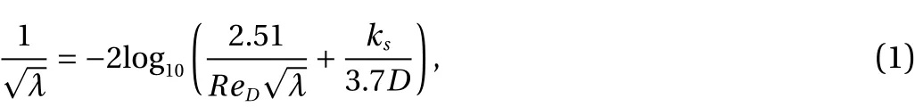
in whichks,ReD, andλrepresent the equivalent sand roughness,the Reynolds number and friction factor respectively. The diameter used in the above correlation is the effective diameter of each phase.ReDis found based on average phase velocity and effective phase diameter

whereρf,µf,Def, andUfare density, viscosity, the effective pipe diameter and mean velocity of the phasefcalculated in the following section. Using the friction factor and mean velocity the shear stress is given by

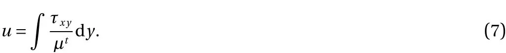
The mean velocity is calculated from the velocity distribution. The velocity profile is obtained using the shear stress correlation

Fig. 1. Schematic of pipe parameters.

By substitution of the above correlation in Eq. (4), the shear stress is

The velocity distribution is obtained by integrating the shear stress achieved in Eq. (6)

The following correlations have been proposed in Ref. [19] in order to findτxyandµt

whereR,Yandu*represent the ratio of the interface to wall shear stress, height ratio and wall friction velocity respectively

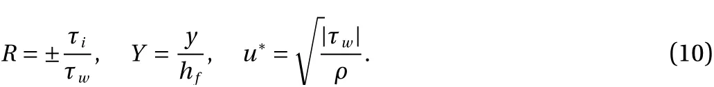
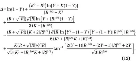
According to Fig. 1, the negative and positive signs ofRare for liquid and gas phases respectively.Kis the dimensionless interfacial turbulence parameter discussed in the next section.Substituting of Eqs. (8) and (9) in Eq. (7) and integrating it gives

in whichκis Stefan-Boltzmann constant. Δ is given by

The integration constantCcould be found by matching Eq. (11)with the wall-bounded velocity distribution [19]. In turbulence theory, the logarithmic velocity distribution for wall-bounded flows is

yielding

in which

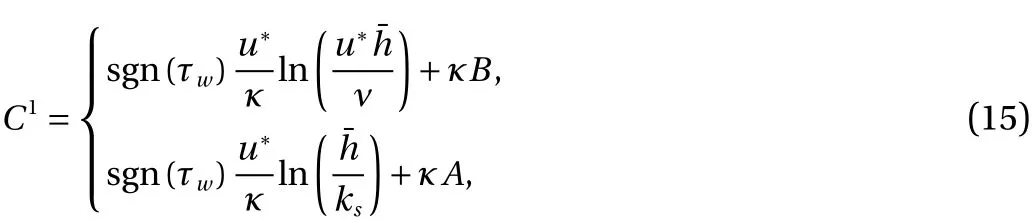
for hydraulic smooth and rough flows, respectively.Ψis

The mean velocity is determined from the following equation

Integrating Eq. (17) gives

in which

Interfacial turbulence parameter is defined byK=li/(κh) in whichliis the mixing length at the interface. Biberg [19] obtained formulas forKfrom the experimental data

for the smooth interface and small waves and

for large waves.

The proposed interfacial turbulence parameters are empirical correlation found from the interpolation of experimental data.

In this paper, these parameters are found from the mean velocity correlation. These parameters are derived by equating the mean velocity obtained from Eq. (18) to the experimental velocity.

The friction factor is a function of Reynolds number. The specific length used inReDis the effective pipe diameter of phasef. This length plays a very important role in calculation of the friction factors. The effective pipe diameter is found from the hydraulic diameter of each phase. Biberg [19] assumed each phase can be considered as a combination of free surface and poiseuille flows. The effective pipe diameter for poiseuille and free surface flow are found from the famous hydraulic pipe diameter formula

in which indicesPandFdenote Poiseuille (R= 1,K= 0) and free surface (R= 0,K≈ 0.5) flows respectively. Using the above correlations, Biberg [19] proposed that the effective pipe diameter of each phase is found from

where

As is clear, in the semi-empirical model, most of the equations are only functions of two dimensionless parametersRandK.SwfandSiare wetted perimeters found from the following.

In order to calculate each phase effective pipe diameter, the wetted perimeters are required to be calculated. The interface morphology has a substantial effect on these parameters. Since at relatively high liquid and gas velocities, the interface does not remain flat, in this paper the interface curvature is taken into account. The interface curvature is modeled using the double circle method [20)]. Figure 2 shows the schematic of this model.

Fan [20] proposed the following equation to find the wetted angle shown in Fig. 2

where

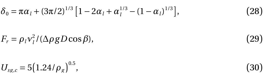
whereFr,Usg,Usg,c,σw,σl,αlandδ0are Froude number,superficial gas velocity, critical superficial gas velocity, water surface tension, liquid phase surface tension, the liquid hold-up and the wetted angle with assuming the flat interface respectively. ConstantsaandC1are

Cross section area of phasefis given byAf=αfA. Void fraction and liquid hold-up are defined byαgandαlrespectively. The gas and liquid-phase wetted perimeters can be calculated using below equations

whereDis the diameter of circle centered atO. In the doublecircle model, the interfacial perimeter is given by

in whichDiandδiare diameter and the wetted angle of circleOifound from

Fig. 2. Geometry of the double-circle model [25].

Fig. 3. Parameters in the double-circle model [25].

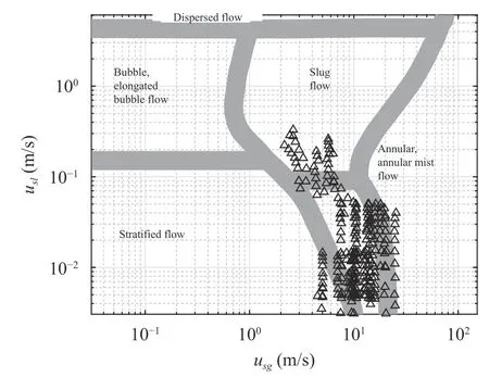
Fig. 4. Applied experimental data on the flow pattern [26].

Table 1 Experimental conditions

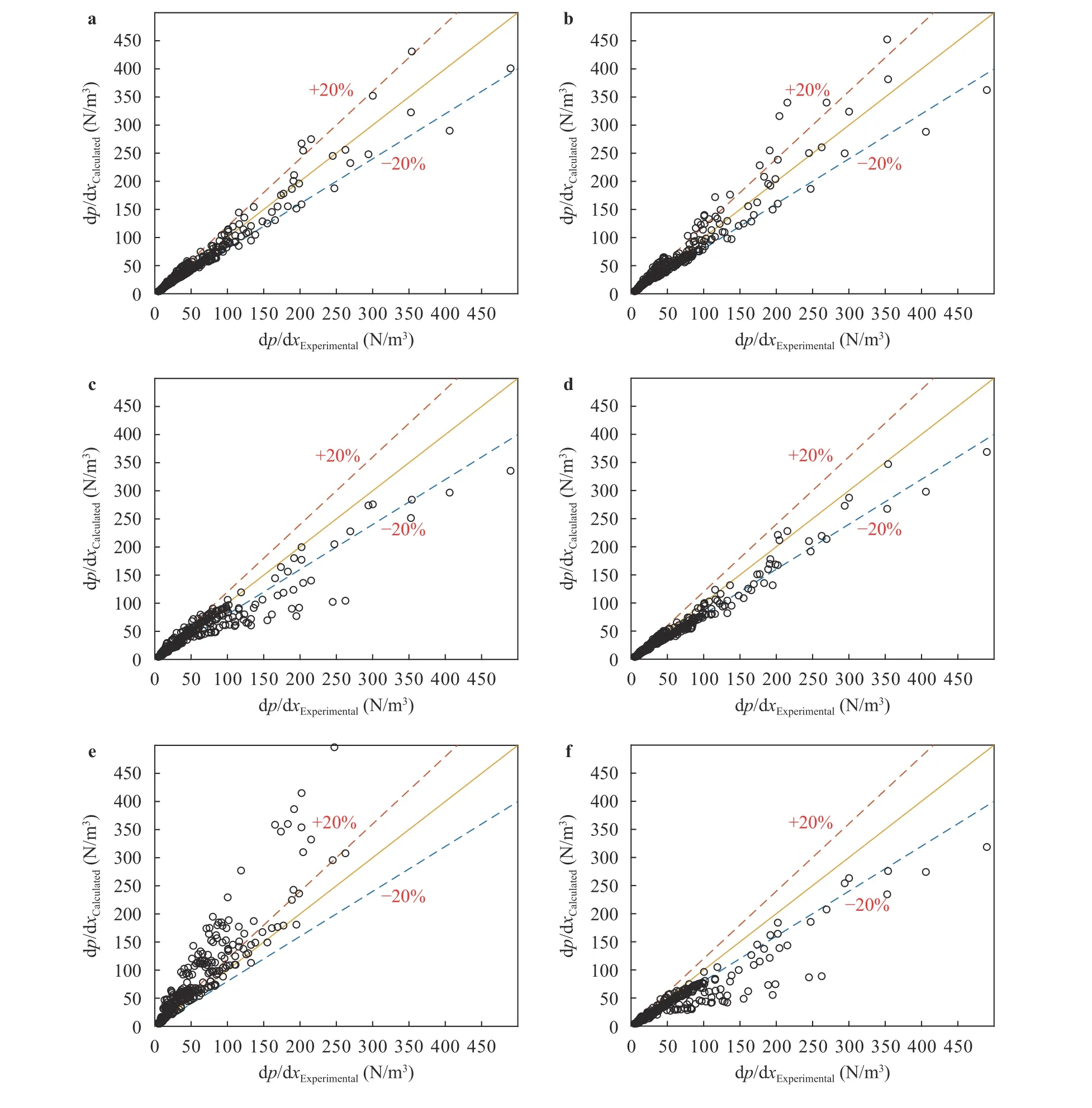
Fig. 5. Pressure gradient comparison (all experimental data). a Present work, b Biberg model [19], c liquid-wall friction factor [12], d Blasius liquid-wall friction factor [1], e Spedding and Hand [9] liquid-wall friction factor, and f Kowalski [6] liquid-wall friction factor.

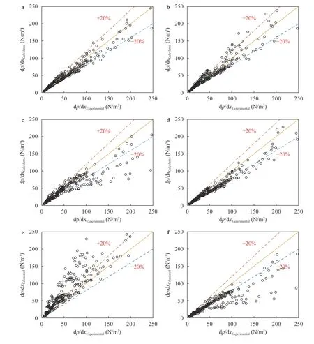
Fig. 6. Pressure gradient comparison (experimental data in 0-250 N/m3 region). a Present work, b Biberg model [19], c Hart et al. [12] liquidwall friction factor, d Blasius liquid-wall friction factor [1], e Spedding and Hand [9] liquid-wall friction factor, and f Kowalski [6] liquid-wall friction factor.

Table 2 Absolute average errors between experimental and predicted pressure gradients

δiis calculated using an iterative solution.

Liquid height (Fig. 3) is found from

where

The average liquid height is given by integrating Eq. (38) with respect to the wetted angle

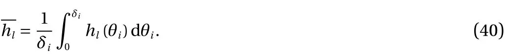
The average gas height is

In this study, the unknown parameters areRg,Rl,KgandKl.The known parameters areUf,αl,D,ρf,µf,ksandβentered into the model from experimental data. In order to find the unknown dimensionless parameters, the equations mentioned below are solved sequentially using an iterative method applied in a computer code until convergence.

The no slip condition on the interface (Y= 0) is used to findRg. This condition is obtained by equating the liquid and gas velocities on the interface from equation Eq. (11)

in this correlation the constantCin the velocity distribution (Eq.(11)) is substituted from mean velocity distribution (Eq. (18)).

Interfacial turbulent parametersKgandKlare found from mean velocity distribution (Eq. (18)). In other words, experimental and calculated mean velocity must be equal in each phase.

Rlis computed from

The wall and interfacial shear stresses in the above correlation are found from Eq. (3) andτi=Rgτgrespectively. The friction factor and the mean velocity in Eq. (3) are calculated from Eqs.(1) and (18). The friction factor is a function of the effective diameter (De) and the Reynolds number (Eq. (2)). The Effective diameter is obtained from Eq. (25) using the wetted perimeter and cross section area. The liquid wetted angle is obtained from Eq. (27). The gas, liquid and interfacial perimeters are calculated form Eqs. (33)-(35), respectively. When the solution is converged, the pressure gradient is derived from two-fluids model under the equilibrium condition.

The model is validated against vast experimental data including Refs. [14, 20-23 ] shown in Fig. 4. The superficial gas and liquid velocities vary from 2.16 m/s to 25.34 m/s and 0.0005 m/s to 0.33 m/s respectively (Table 1).

The pressure gradient obtained from the present model is compared with a combination of different empirical correlations (Blasius [1], 12, 6 and 9). The results are shown in Fig. 5 for all of the experimental data.

In order to make the results more visible, as most of the experimental pressure gradients are less than 300 N/m3, Fig. 6 shows the validated data in this region. The results show that the present model is in good agreement with experimental data in comparison with other models.

The absolute average error (AAE) defined in Eq. (45) is used to quantify the deviation of the theoretical data from experiments

Fig. 7. Pressure gradient validation by taking various gas-wall friction factors in the present model: a Colebrook et al. [5], b Blasius [1]and c Taitel and Dukler [3].

Table 3 AAE for three different gas-wall friction factor

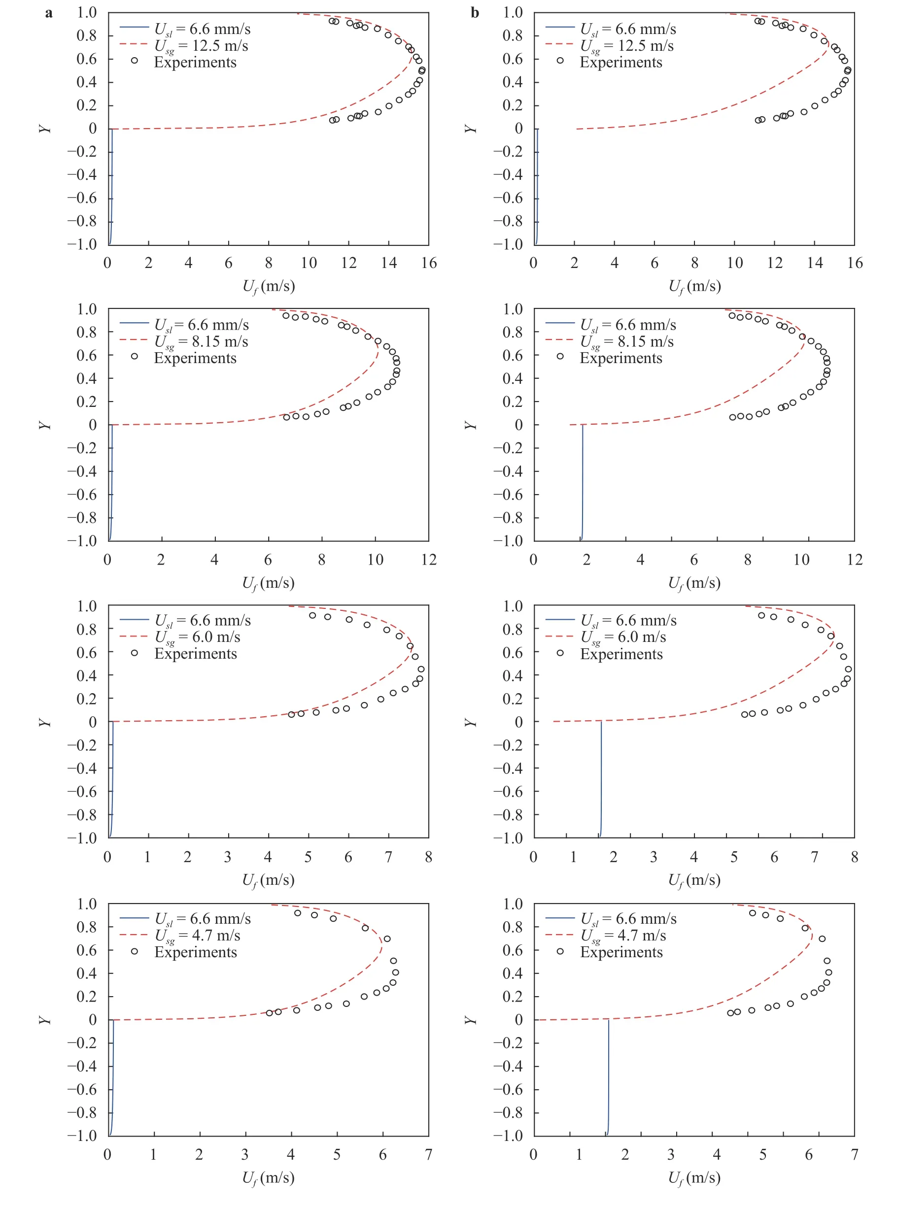
Fig. 8. Comparison of velocity distribution of gas and liquid phases against Lopez [27] experiments. a Present work and b Biberg [19].

in whichMnandPnare measured (or correlated) and predicted values, andNthe total number of experiments.

According to the pressure gradient diagrams, the present semi-empirical model improves the absolute average error of the semi-empirical model by 3% [19].

In all of the empirical models employed to predict the pressure gradient in Figs. 5 and 6, the gas-wall and interfacial friction factors are used [3]. However the effects of the gas-wall friction factor on the pressure gradient is examined in the following section.

The absolute average errors of the data shown in Fig. 6 are in Table 2.

In this section, the effects of gas-wall friction factor on the pressure gradient is evaluated by employment of three different gas-wall friction factors in the present model [1, 3, 5].

As shown in Fig. 7, different gas-wall friction factors provide approximately the same results. This approves that all of these models can precisely predict the gas-wall shear stress.

The absolute average errors of data in Fig. 7 are shown in Table 3.

As mentioned in the previous sections, one of the disadvantages of Ref. [19] semi-empirical model is that the gas and liquid velocities are not the same on the interface. In the present work,in contrast to Biberg model [19] the interfacial turbulence parameters are found by equating the mean velocity profile (Eq. (18))to the experimental velocity.

The gas and liquid velocity profiles predicted from the present and Biberg [19] models are plotted in Fig. 8. The results are validated against experimental data of Ref. [27]. As shown in Fig. 8, the gas and liquid velocities are not the same at the interface in Biberg model [19]. However in the present model, the interfacial gas and liquid velocities are equal. Moreover, the gas velocity profile is closer to the experimental data in the present model.

An improved semi-empirical model is introduced in this paper based on the modification of the model proposed by Biberg[19]. In contrast to the Biberg model [19], where the interfacial turbulence parameters have been found based on experimental data, they are found by equating the mean velocity profile (Eq.(18)) to the experimental velocity. By this modification, the model dependency on the experimental conditions decreases and also the no slip condition on the interface is satisfied. Since at relatively high liquid and gas velocities, the interface does not remain flat, the interface curvature is also taken into account.

A comprehensive comparison between the present semi-empirical model and other empirical correlations is performed using vast experimental databases [14, 20-23]. Comparisons show that the proposed semi-empirical model is in better agreement with the experimental data compared to the empirical correlations available in the literature. By increasing the phases velocities, this superiority will be more evident.

Thus by application of the proposed modifications in the original model, the resulted pressure gradient absolute average error diminishes about 2.5%; the attained velocity profile becomes closer to the experimental data and the no-slip condition is satisfied at the interface.

Acknowledgement

This work was supported by the Iran National Science Foundation (Grant 96006257).