Numerical solution for a semilinear parabolic blowup-combustion model
2020-06-03YangHongbinXuYufeng
Yang Hongbin Xu Yufeng
(1.School of Mathematical Sciences, Nankai University, Tianjin 300071, China;2.School of Mathematics and Statistics, Central South University, Changsha 410083, China)
Abstract In this paper, we study an efficient finite difference method based on the uniform mesh for a class of semilinear parabolic equation arising from combustion process.Due to the capability of exponential source on simulating Arrhenius reactive rate, the considered model may theoretically describe the rigid ignition process in combustion.By introducing an indicator, the original equation is transformed to an approximate model with globally smooth solution.When the cut-off level constant is sufficiently large, the solution of original equation can be obtained by solving the approximate model, without numerical blowup.By carefully choosing the step sizes, the blowup position and moment can be computed more simply and efficiently.Finally, numerical simulations are provided to verify the mathematical analysis and physical properties of proposed blowup-combustion model.
Key words Semilinear parabolic equation Finite difference method Exponential source Monotonicity Cut-off level function
1 Introduction
In practice, a combustion process may involve a large number of different complex physical and chemical reactions which are apparently to be observed but difficult to be described in concise mathematical models.In the recent decades, the following homogeneous Dirichlet boundary value problem of seimilinear partial differential equations has attracted considerable attention[1]
(1)
whereδ>0 is called the Frank-Kamenetskii constant,L>0 is the length of spatial domain,u0is the initial heat distribution, andu(x,t)usually shows the desired temperature at particular positionxand momentt.Here we only consider a one-dimensional case.Nevertheless, for some real combustor with radial symmetry, it can be well-described by such an equation qualitatively.For rigid ignition model(1), it is well-known that there is a critical valueδ*>0 such that
(1)ForδL>δ*,the classical solution of model(1)will cease to exist after a short period of time.That means, there is aTb<∞,such that
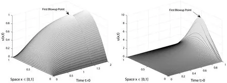
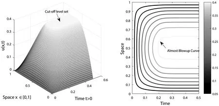
(2)Forδ<δ*,the classical solution of model(1)is bounded and globally well-defined for all 0 The initial study of model(1)may date back several decades ago.With the aid of physical and chemical theories, mathematical models for combustion process become more and more realistic[2].In general, combustion is a complicated phenomenon companying many physical and chemistry reactions.By using mass and energy conservative laws, several parabolic, hyperbolic and mixed versions of both are established[1,2].Thanks to the development of the Frank-Kamenetskii theory, which explains the thermal explosion of a homogeneous mixture of reactants, kept inside a closed vessel with constant temperature walls(it is named after a Russian scientist David A.Frank-Kamenetskii, who along with Nikolay Semenov developed the theory in the 1930s), the original tanglesome source term is finally simplified as the exponential type, since a key assumption that the reaction rate governed by Arrhenius law is applied[3,4,5].Later on, due to observations in more experiments, another source term is of power-law type(f(u)=|u|p-2uwithp∈(2,2#),where 2#is named as the critical Sobolev exponent)also receives extensive attention[6]. In theoretical field, semilinear elliptic equations and parabolic equations with exponential sources have been studied extensively in the recent years.Various of existence and regularity results are obtained by variational methods, topological arguments, and some particular nonlinear analysis techniques.For instance, in[7], the author again pointed that problem(1)arises in the theory of thermal self-ignition of a chemically active mixture of gases in a vessel.Further, it has proved a certain relationship among solutions of problem(1)and its stationary equation(∂tu≡0), which shows that classical solutions of(1)will converge to solutions of the associated stationary problem under certain assumptions.To be more specific in modelling, a general nonlinear sourcef(u),which is smooth, positive, increasing, and strictly convex, can be considered in problem(1). In numerical field, the development is equally wonderful.In the early stage, finite difference scheme based on uniform mesh for(1)are extensively investigated, see[8,9].Later on, it becomes more popular in imposing moving mesh method and variable step size technique[10,11,12,13].Recently, with the help of theoretical results on the existence and structure of classical solutions, it is possible to construct more efficient numerical methods which are physical-preserving and structure-preserving[14,15].Surely, this is important to solve models with blowup phenomena, where the moment, place and profile of blowup solution are usually crucial in real-world problems. There is one more interesting phenomenon called complete blowup, which means that the blowup set is no longer isolated but takes up a subset of positive measurement of spatial domain, even the whole spatial domain except the boundaries.It seems that only few attention are drawn on this direction, because the complete blowup does not show up simultaneously.It cannot be numerically approximated if we solve the original semilinear PDE by transforming it into a linear algebraic system.In such a away, computation in general fails once the model blows up at the first time.In[16], the occurrence of complete or incomplete blowup is discussed for a general quasilinear heat equation.It is verified that a superlinear source will result in blowup phenomenon within finite time.One may also see that an important issue of blowup problems is the possibility of having a nontrivial extension of the solution after the first blowup appears, i.e., after the singularity occurs.In references, the blowup phenomenon is said to be incomplete if such continuation exists; otherwise, the blowup phenomenon is said to be complete.In[17], The complete blowup for a degenerate semilinear parabolic equation with Dirichlet boundary condition is discussed.It is proved that under certain conditions, the classical solution will blow up in a finite time, and the blowup set will finally reach the entire spatial interval.Motivated by the theoretical conclusions above, we attempt to numerically study the complete blowup for a one-dimensional semilinear parabolic equation.Since the blowup set will eventually occupy the whole domain, there must be a serious boundary layer where the first-order spatial partial derivative changes dramatically in the vicinity of boundaries, once Dirichlet boundary condition is imposed.Therefore, special mesh size is surely needed in numerical simulation to reduce the total computational cost and maintain the high accuracy of approximation. So far as we know, the numerical investigation for blowup phenomenon of mathematical combustion models are still not complete.Especially high-resolution numerical method for first blowup, complete blowup, blowup set and moments deserves further endeavor.Therefore in this paper, we introduce a modified model of(1)by imposing an indicator on source: (2) whereγ≥1 is the cut-off level constant, and Furthermore, we could again simplify model(2)by applying scale transform.That is, letu(x,t)→u(Lx,L2t),then we have (3) whereδL=L2δ.Without loss of generality, we shall focus on the blowup places, blowup time and complete blowup of the above combustion model by using the standard finite difference scheme.Besides, the positivity, monotonicity and global/local existence of classic solution for combustion model will be discussed. The remainder of this paper is organized as follows.In Section 2, we carry out some mathematical analysis on local and global existence results for Model(1)and Model(3).The blowup time for Model(1)will be estimated by using Kaplan’s principle eigenvalue method.In Section 3, numerical method and analysis will be given, and the finite difference scheme based on uniform mesh and non-uniform mesh will be studied.In Section 4, numerical experiments are shown to validate the theoretical analysis in previous sections.Finally, conclusions will be summarized in Section 5. In this section, we will briefly recall the existence, uniqueness and blowup properties of the classical solution of model(2), which play significant roles in design of suitable numerical method in simulation. We shall discuss the existence, uniqueness and regularity of the mild solution of model(2).Multiply equation of model(2)byφ(x)on both sides, and integrate with respect toxon[0,L],to give that (4) whereφ(x)solves the following eigenvalue problem, φ″(x)+λφ(x)=0,φ(0)=φ(L)=0. Denote a projection ofuby (5) then(4)implies that (6) (7) Solving the differential inequality above leads to (8) Asγapproaches infinity, the lower bound oftconverges to zero.This indicates the global existence of solution of model(2). Let us firstly study the finite difference scheme for(3)on a uniform mesh.We begin with some basic definitions and notations.Due toδL>δ*,the classical solution of model(3)will blow up within finite time as shown in previous references[1,7].Now we considerT*=Tb-ε,whereε>0,thenu=γby the assumptions.With the above preparations, model(3)reduces to (9) Now, we introduce some difference operators Moreover, lettinglh={xj|0≤j≤J},Vh={u|u={uj|0≤j≤J},u0=uJ=0},which allows us to define a discrete inner product for anyu,v∈Vh, Then, some equivalent induced norms are written as which leads to (10) By a combination central finite difference method(Crank-Nicolson scheme),(10)becomes (11) wherej=1,2,…,J-1. Theorem 3.1The local truncation error of scheme(11)reads (12) whereτandhare respectively the temporal and spatial step sizes. which immediately give Summing them together gives Physically, it is not difficulty to observe that asugrows, the temperatureugoverned by combustion model will increase gradually due to the effect of exponential source term.Next, we show that the discrete scheme admits monotonicity property. ProofBy(11), we get (13) The eigenvalue ofAreads which shows thatτA(Un+1+Un)is bounded from above and from below for allUn∈RJ-1.Therefore, whenτis sufficiently small andδLis large enough, one may easily deduce that the right hand side of(13)is non-negative. We continue to discuss the convergence of the numerical scheme. and ProofThe proof is direct and trivial.Similar result may be found in even textbook of numerical analysis. Theorem 3.4LetT*be any moment before first blowup of model(1).Then the error estimate up to this particular time layer is governed by (14) whereCis a constant independent of step sizes. (15) Subtract(11)from(15), to give (16) (17) The above calculation is obvious, and only the simplification of the product of the first item at the right end of Equation(17)is explained. Next, we carry out estimate for(17).By assumption,|u|≤γ,therefore, which transforms(17)into (18) (19) Finally, we study the stability of the difference scheme.Here we focus on the stability on the initial condition. ProofWe assume bothu1andu2are classical solutions depending on the initial conditionsφ1andφ2.Letu=u1-u2,φ=φ1-φ2.We arrive at (20) Similarly, we have (21) In this part, we first present blowup phenomenon at a single point by using the finite difference method discussed above.Then we use the explicit iteration method to obtain the complete blowup for the considered model.Inspired by the theoretical results on the bifurcation of the Gelfand equation, we are interested in numerical simulations of the considered model withδ≠3.5,sinceδ=3.5 is a turning point in the bifurcation diagram of the 1D Gelfand equation.For the purpose of easy-to-compute and illustration, we impose a cut-off level as stopping criterion to simplify the total computation process. Whenδ=3.5 andγ=1,the numerical solution of model(2)are presented in Figure 4.1.One may observe that once the original model is approximated by the resulting linear system, and whenever the maximum norm of the approximate solution approachesγ,the exponential source is down to zero immediately, which leads the numerical solution decreases for a while and then again grows rapidly due to the impaction of the exponential source term.Those oscillations can be constantly viewed if computational time is relatively long. Meanwhile, we setδ=4.05 andγ=10.We see that in the vicinity of the only blowup point, say(x,t)≈(1/2,0.98),both the temporal derivative and spatial derivative ofu(x,t)are greater than those of the first case which are shown in the right part of Figure 4.1.This can also be regarded as an evidence of monotonicity for the solution of model(2). Figure 4.1 Numerical simulation near blowup moment(Left: δ=3.5, γ=1; Right: δ=4.05, γ=10) Figure 4.2 Numerical illustration for almost complete blowup phenomenon(Left: Numerical solution with cut-off level; Right: Contour plot for the corresponding 3D outputs.) Finally, with the help of the Jacobian iteration, we are able to calculate all the function values under the cut-off level.When the parameter of the cut-off level function becomes sufficiently large, one may regard the combustion model arrives its complete blowup state.At this stage, all the solutions become infinity.Nevertheless, to just give an illustration, we take the parameterγnot too large for the reasonable scale of outputs.In Figure 4.2 below, we can see that the contour plot clearly exhibits the cut-off level, and all the function values eventually approachγ=0.4,although those from the neighborhood of boundaries grow slowly.Abstractly, we could know that the blowup set of this case is not of measure zero.While in the last output, the numerical calculation will fail for the first time when the first blowup point appears. In this paper, we studied a class of diffusion equation with exponential source arising from combustion processes.An important character of this model is that its solution ceases to exist whenever the parameter(associated with the exponential source)exceeds the threshold, under suitable selections of the domain size and initial condition.As an abstract combustion model, we investigated its physical property such as positivity, monotonicity and almost complete blowup, by imposing a cut-off level.In numerical simulation, a direct finite difference scheme with second-order accuracy is applied on uniform meshes.However, such a computational idea may be extended to non-uniform meshes or other structural grids.To improve the computational efficiency, we intend to study two and three dimensional combustion models by using multi-level solvers in the future work.2 Theoretical results
3 Numerical methods and analysis


4 Numerical Simulations and Discussions
5 Conclusions