Atmospheric responses over Asia to sea ice loss in the Barents and Kara seas in mid–late winter and early spring: a perspective revealed from CMIP5 data

HAN Zhe & LI Shuanglin

Atmospheric responses over Asia to sea ice loss in the Barents and Kara seas in mid–late winter and early spring: a perspective revealed from CMIP5 data

HAN Zhe1*& LI Shuanglin2,3

1CAS Key Laboratory of Regional Climate-Environment for Temperate East Asia, Institute of Atmospheric Physics, Chinese Academy of Sciences, Beijing 100029, China;2Nansen-Zhu International Research Center (NZC), Institute of Atmospheric Physics, Chinese Academy of Sciences, Beijing 100029, China;3China Univercity of Geosciences, Wuhan 430074, China

This study investigated atmospheric responses in mid–late winter and early spring to sea ice loss in the Barents and Kara seas using regressions of the January–March mean atmosphere on Barents and Kara sea ice area in November and December. Similar atmospheric circulation responses were obtained from reanalysis data and multimodel ensemble results from the Coupled Model Intercomparison Project Phase 5, i.e., sea ice anomalies are the dominant factor driving the overlying atmosphere. The results showed that an Arctic–Asia dipole structure, with opposite anomalies over the mid-latitudes of Asia and over the adjoining Arctic, appears to be the key atmospheric circulation anomaly influencing the East Asian climate in mid–late winter and early spring.

winter atmospheric circulation, Arctic–Asia dipole, sea ice loss, Barents and Kara seas

1 Introduction

As an important part of Earth’s climate system, Arctic sea ice can modulate oceanic–atmospheric heat, moisture, and momentum exchanges and it can act as an important driver of climate on interannual–interdecadal timescales (Honda et al., 1999; Wu et al., 1999; Alexander et al., 2004; Magnusdottir et al., 2004). Observational analyses have suggested the sea ice in the Barents and Kara (B–K) seas is closely connected with the Asian climate (e.g., Honda et al., 2009; Wu et al., 2011; Mori et al., 2014; Zuo et al., 2016). These previous studies focused mainly on the winter (December–February) climate. Although a few studies have investigated the January–March (JFM) mean atmospheric response to sea ice (Kim et al., 2014; Yang et al., 2016), they have tended to focus on the zonal mean circulation and they have not provided spatial details of the atmospheric circulation anomalies over Asia. Moreover, Kim et al. (2014) focused on the long-term trend instead of the seasonal–interannual variability. Therefore, the climate in mid–late winter and early spring (i.e., JFM) needs to be studied further. In addition, there could be large uncertainty in observational analyses because of the short-term period of investigation (Simmonds and Govekar, 2014; Vihma, 2014; Walsh, 2014; Overland et al., 2016). To overcome these disadvantages, this study used the historical experiments in nine models from the Coupled Model Intercomparison Project Phase 5 (CMIP5). This approach involved the consideration of long-term data series (about 150 a for each model simulation), while the use of nine models reduced the uncertainties attributable to model deficiencies.

As in previous studies, the observed atmospheric response to the Arctic sea ice anomaly in winter was obtained by investigating its lagged correlation with Arctic sea ice in the previous season (e.g., Honda et al., 2009; Wu et al., 2011; Mori et al., 2014). This is because the simultaneous relationship between oceanic and atmospheric anomalies mainly reflects the forcing role of the atmosphere on sea ice (e.g., Deser et al., 2000; Wu and Zhang, 2010; Han et al., 2016). In the present study, we also used the JFM mean atmosphere lagged sea ice in November–December (ND) to indicate the atmospheric response to sea ice loss in the B–K seas. We did not use the JFM mean atmosphere lagged sea ice loss of the previous autumn (e.g., September) because the area of significant winter sea ice forcing in the B–K seas that persists from the previous autumn (especially September) is smaller than that of ND. This is because sea ice variation in the B–K seas is greater in ND than in autumn, and because greater heat anomalies are released to the atmosphere over a longer period of forcing. Thus, for equivalent sea ice anomalies, those persisting from autumn are weaker than those persisting from ND. In general, strong external forcing will produce a strong atmospheric response and thus the results could be considered more credible. This is confirmed by the results of simulations from CMIP5, which show that the longer sea ice anomalies drive the atmosphere, the weaker the sea ice anomalies are (Figures 1a and 2c). This weakens the surface energy exchange (Figures 1b and 2d) and thus the atmospheric responses become weaker (Figures 1c, 1d, 3c, 3d). Under limited observational samples, the stronger the oceanic forcing is, the more credible the results are. Therefore, the use of ND rather than autumn has tangible advantages. The physical basis of oceanic–atmospheric interaction in reanalysis data and coupled models is introduced in section 2. Aside from the reanalysis data, to enhance reliability, we also used nine CMIP5 models to investigate this subject. The findings of this study could be helpful in understanding the relationship between the strengthening of the Siberian High (Jeong et al., 2011; Wu et al., 2011; Zhang et al., 2012) and the loss of sea ice in winter in the B–K seas over the past two decades.

Figure 1 CMIP5 JFM mean sea ice (SIC, shaded, %) and sea surface temperature (SST, contour, ℃, a), surface turbulent heat fluxes (SLH, W·m−2, b), monthly sea level pressure (SLP) (hPa, c), and Z500 (gpm, d) regressed on the sign-reversed September–October B–K sea ice area (SIA) index. Black contours indicate significance at the 95% level.

2 Data and methods

The monthly sea ice concentration and SST data used in this study were obtained fromthe UK Meteorological Office’s Hadley Centre (Rayner et al., 2003). The SLP, 500 hPa geopotential height (Z500), surface air temperature (SAT), and surface turbulent heat fluxes (sensible and latent heat fluxes) were obtained from the European Centre for Medium-Range Weather Forecasts’ Interim Reanalysis (Dee et al., 2011). The snow cover data were obtained from the National Snow and Ice Data Center (Brodzik and Armstrong, 2013). The North Atlantic Oscillation (NAO) index was taken from NOAA’s Climate Prediction Center. The period after 1979 was used for the analyses because of the relatively higher quality of the sea ice data in comparison with earlier years. Specifically, the period 1979–2016 was used, except for snow cover, for which the period of analysis was 1979–2015. First, the monthly seasonal cycle of 1979–2016 was removed for all variables and then the linear trend was removed. In this study, the Siberian High was defined as the mean SLP within the region 40°–60°N, 80°–120°E. Variations of sea ice in the B–K seas were represented by a sea ice index, defined as the SIA in the B–K seas (60°–85°N, 5°–90°E). The JFM period was considered to represent mid–late winter and early spring.

Figure 2 JFM SIC (shaded, %; a, c) and SST (contours, ℃; a, c), SLH (W·m−2; b, d) regressed on the sign-reversed ND B–K SIA index. The results shown in a and b are from reanalysis data, while b and d are from CMIP5 simulations. Panels e and f are the same as c and d, except they are regressed on the SST-independent ND B–K SIA index, which is the B–K SIA index after removal of that linearly related to the SST index, which is defined as the difference between area-averaged SST over the domains 51°–65°N, 60°–5°W and 32°–48°N, 60°–5°W. Contour intervals are 0.2 ℃in a and 0.1 ℃ in c and e. Black contours indicate significance at the 95% level.

Figure 3 ND mean SLP (hPa; a, c, e) and Z500 (gpm; b, d, f) regressed on the sign-reversed ND B–K SIA index. The results shown in a and b are from reanalysis data, while those in b and d are from CMIP5 simulations. Panels e and f are the same as c and d, except they are regressed on the SST-independent ND B–K SIA index, which is the B–K SIA index after removal of linearly related to the SST index, which is defined as the difference between area-averaged SST over the domains 51°–65°N, 60°–5°W and 32°–48°N, 60°–5°W. Contour intervals are 0.2 ℃ in a and 0.1 ℃ in c and e. Black contours indicate significance at the 95% level.

Nine CMIP5 models were used (Table 1) and each model comprised three ensembles. The only difference between the ensembles of each model was the initial conditions. The period of CMIP5 data used for the analysis was 1946–2005. A nine-year running mean was subtracted to remove interdecadal variability; thus, the remaining data reflected interannual variability during 1950–2001. Finally, we had a large sample of 153 years’ data for each model. To a large extent, more samples can eliminate the influence of atmospheric internal variability, which has strong influence on the atmospheric response to oceanic forcings (e.g., Mori et al., 2014; Screen et al., 2014). However, as the reanalysis data spanned only 38 a, the sample size would have been very small if the interdecadal variability had been removed by subtracting the nine-year running mean. Thus, we only removed the linear trend, which meant the remaining data approximately reflected the interannual variability. This method has been used in most previous similar studies (e.g., Honda et al., 2009; Wu and Zhang, 2010).

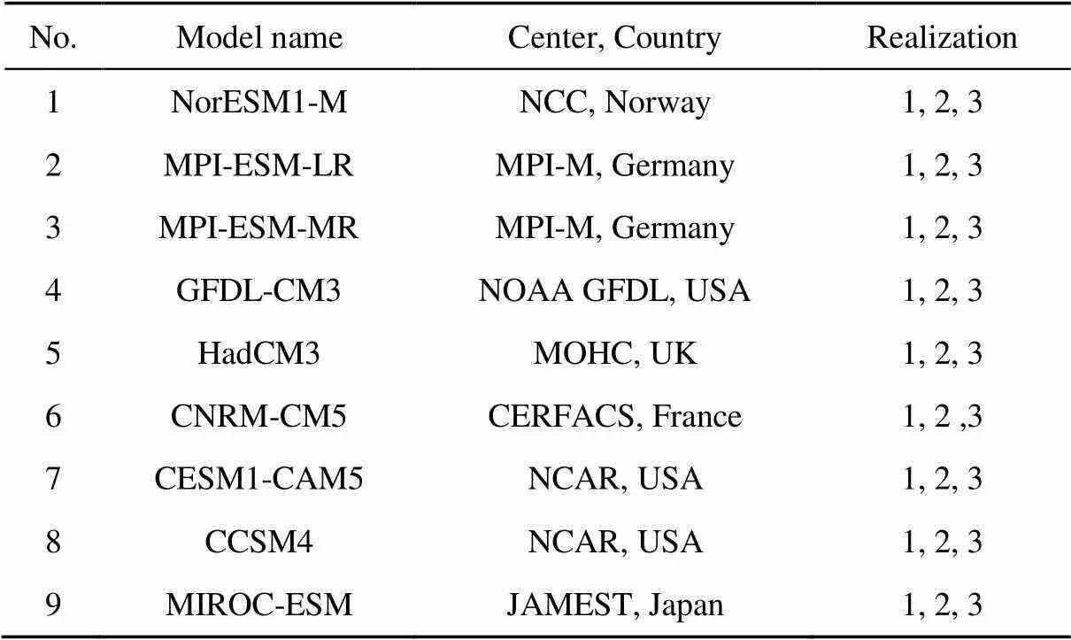
Table 1 List of nine CMIP5 models used in this study

In this paper, the atmospheric response to a sea-ice anomaly in the B–K seas in JFM is defined as the regression of the JFM mean atmosphere on the ND mean B–K SIA. The physical basis for this is as follows. When sea ice anomalies are present in the B–K seas in ND, there might be atmospheric circulation anomalies in the following JFM. Therefore, if there are atmospheric circulation anomalies in JFM, it is important to determine their cause. Many previous studies have indicated that the persistence of the intrinsic atmospheric circulation at mid–high latitudes endures for no longer than one month (e.g., Gastineau et al., 2013; Frankignoul et al., 2014); thus, the atmospheric circulation at mid–high latitudes cannot persist from ND to JFM. In other words, the atmospheric circulation anomalies in JFM bear no relation to those in ND, which appear simultaneously with B–K sea ice anomalies in the same period. Therefore, the most plausible reason for the existence of atmospheric anomalies in JFM is that they are caused by another external driver that can persist for a relatively longer time. In this respect, oceanic anomalies are a likely possibility. For example, sea ice anomalies occurring in ND could exist continuously through to the following JFM because they involve huge heat content anomalies. In summary, the lagged regression of the atmosphere on sea ice might indicate an atmospheric response to sea ice, and many previous studies have used this method to study the atmospheric response to oceanic anomalies (e.g., Czaja and Frankignoul, 2002; Honda et al., 2009; Wu and Zhang, 2010; Strong et al., 2011; Liu et al., 2012). Importantly, the atmosphere lags the sea ice by more than one month (Strong et al., 2011; Frankignoul et al., 2014). If the lag time were less than (or only) one month, any so-called atmospheric response might be strongly impacted by the persistence of the atmosphere. For example, Inoue et al. (2012) used the lagged relationship between sea ice in December and the atmosphere from December– February to indicate the atmospheric response. However, because the lag time was only one month, the atmospheric response was insignificant over the North Atlantic, and it was very different to the positive NAO-like circulation response indicated in previous studies (e.g., Magnusdottir et al., 2004; Strong et al., 2011; Liptak and Strong, 2014; Wu et al., 2015).

The question to be addressed is whether SST and sea ice anomalies are forcing of or responses to the overlying atmosphere. In general, if a warm SST (atmospheric) anomaly were forcing an atmospheric (SST) anomaly, there would be significant upward (downward) heat fluxes. Conversely, if a cold SST (atmospheric) anomaly were forcing an atmospheric (SST) anomaly, there would be significant downward (upward) heat fluxes. However, the relationship between sea ice and surface heat fluxes is somewhat different, as explained in section 3.

3 Results

3.1 Reanalysis data

3.1.1 Roles played by sea ice and SST anomalies

First, we examine whether the sea ice anomaly, obtained based on the method introduced in section 2, is the dominant oceanic forcing driving the atmosphere in winter. When there is significant sea ice loss in ND (shading in Figure 4a), the sea ice anomaly can persist into JFM (shading in Figure 2a), and such a slow change can be seen clearly in Figure 2c of Strong et al. (2011). During ND, the sea ice anomaly is caused mainly by the contemporaneous atmosphere because there are opposite surface heat flux anomalies in the sea ice region and in adjoining open oceans (red and blue boxes in Figure 4b). These opposite surface heat flux anomalies can also be found in the CMIP5 simulations (Figures 4d and 4f). The atmosphere can induce northward advection of warm temperatures and lead to downward surface heat flux anomalies (Deser et al., 2000; Sato et al., 2014; Sorokina et al., 2016; Woods and Caballero, 2016), which is the reason for the opposite surface heat flux anomalies in the Barents Sea. This result is essentially the same as that discussed in the introduction, i.e., the simultaneous relationship between oceanic and atmospheric anomalies in winter mainly reflects the forcing role of the atmosphere on the ocean. However, when the sea ice anomalies persist into JFM, they play a role in driving the atmosphere, as can be seen from the upward surface heat flux anomalies in the areas of sea ice loss and adjoining open ocean regions (Figure 2b).

To further investigate whether sea ice loss is the dominant oceanic forcing, the SST anomalies are examined because they often occur together with sea ice anomalies (e.g., Wu et al., 2011; Han et al., 2016). Such anomalies can persist into the following season and thus they might influence the atmosphere. Figure 4a shows that there are indeed SST anomalies during ND. The correlation coefficient between the SST anomalies and the surface heat flux anomalies is −0.40 over the domain 20°–60°N, 80°W–0°, which suggests a role of atmospheric forcing on the SST anomalies. Moreover, the ND SST anomalies do not persist into the following JFM (color contours in Figures 2a and 4a) when the significant anomalies are present only in the mid-latitudes of the North Atlantic. In contrast to the role of sea ice, the SST anomalies in JFM appear to be caused by the atmosphere because the surface turbulent heat flux anomalies are upward over colder SST regions. In addition, there are no SST anomalies in the tropical Pacific, which is usually an area with important influence on the winter climate over Asia. The above analysis suggests that sea ice anomalies in JFM are mainly the result of oceanic forcings.

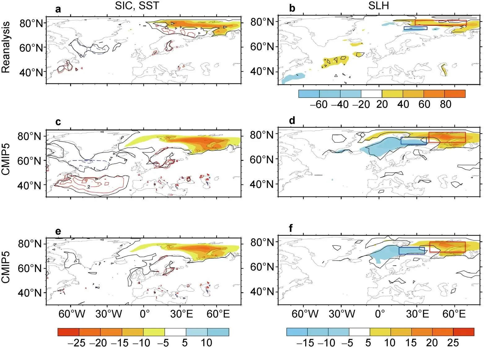
Figure 4 Same as Figure 3 but for (a, c, e) sea ice (shaded, %; a, c) and SST (contour, ℃), and (b, d, f) surface turbulent heat fluxes (W·m−2).

3.1.2 Atmospheric responses

Under sea ice forcing, there are significant SAT anomalies and snow cover anomalies during JFM in Asia (Figures 5a and 5b). This suggests that sea ice loss in the B–K seas has important influence on the Asian climate in mid–late winter and early spring. Next, we investigate the key atmospheric circulation anomalies via which sea ice influences the Asian winter climate. The atmospheric circulation responses to sea ice loss, which are the regressions of JFM mean SLP and Z500 anomalies on the sign-reserved ND mean B–K SIA, are shown in Figures 3a and 3b. There are high-pressure anomalies in the Arctic and high latitudes of Asia and low-pressure anomalies in the mid-latitudes of Asia (Figure 3a). Such north–south pressure differences benefit the transfer of cold air from the Arctic to the mid–high latitudes of Asia, and they lead to cold anomalies over most of that region (Figure 5a). This spatial pattern bears some resemblance to the Asia–Arctic pattern described in Wu et al. (2015), but the important difference is that the anomalies in the mid-latitudes of Asia, reported in Wu et al. (2015), are much weaker than in the high latitudes. Here, we redefine this pattern, identifying it by the second empirical orthogonal function (EOF) of SLP in JFM over the domain 40°–90°N, 60°–150°E. This mode explains 16% of the total variance (Figure 6a), and it is statistically significant according to the criteria of North et al. (1982). Because the anomalies in the Arctic are stronger than in mid-latitude regions, we refer to this pattern as the Arctic–Asia dipole. Using the Arctic as the beginning of the phase shows the importance of anomalies in the Arctic. The correlation coefficient between PC2 and the B–K SIA in ND is 0.39 and it is above the 0.98 significance level (Figure 6c). In addition, the spatial correlation coefficient between Figure 3a and Figure 6a is 0.74 over the domain 40°–90°N, 60°–150°E. Here, we do not show the first EOF because the correlation coefficient between PC1 and the B–K SIA in ND is only 0.18 and it is non-significant. As the pattern of SLP anomalies is largely different from that shown in Wu et al. (2015), the related climate anomalies also have differences, especially in Europe and the low–mid-latitude regions of Asia (Figure 5a in this paper and Figure 4c in Wu et al., 2015). In the middle troposphere, the geopotential height anomalies also show a dipole structure with negative anomalies in East Asia and positive anomalies in the adjoining Arctic (Figure 3b). The Siberian High response to sea ice loss in JFM is very weak (40°–60°N, 80°–120°E; Figure 3a), i.e., the anomalies in the Siberian High region are non-significant and they are opposite in north and south regions of the Siberian High. The correlation coefficient between the JFM mean Siberian High index and the ND mean B–K SIA is 0.00 (Figure 6d). This is different from the winter atmospheric response to sea ice found in previous studies (e.g., Honda et al., 2009; Wu et al., 2011; Mori et al., 2014), in which a significant Siberian High anomaly was reported, and the reason might be related to the different atmospheric background. Previous studies have suggested that atmospheric responses are sensitive to the atmospheric background (Peng et al., 1997; Li, 2004).

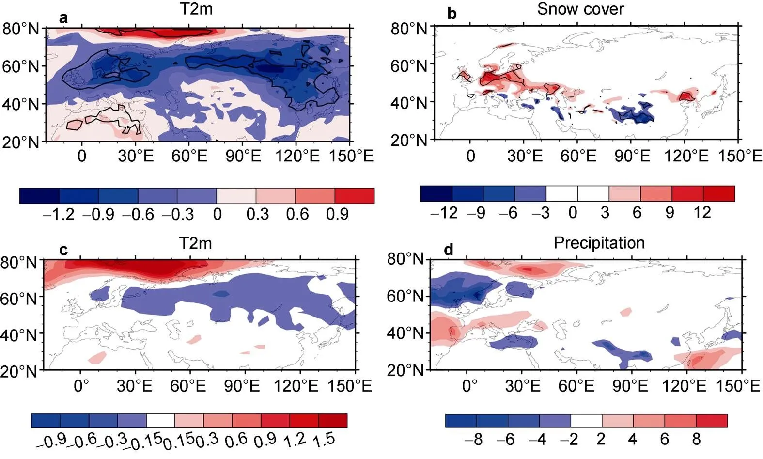
Figure 5 JFM mean SAT (℃, a) and snow cover (%, b) regressed on the sign-reversed ND B–K SIA index. Nine-model ensemble mean SAT (c) and precipitation (d) in JFM regressed on the sign-reversed ND B–K SIA index. Black contours indicate significance at the 95% level.

Figure 6 Second EOF of monthly SLP in JFM over the domain 40°–90°N, 60°–150°E: ERA-Interim (a) and multimodel CMIP5 experiments (b). Scatter plot of JFM mean Arctic–Asia index vs. ND mean B–K SIA index (c). Scatter plot of JFM mean Siberian High index vs. ND mean B–K SIA index (d). Contour interval in a, b is 1 hPa; negative values shown by dashed lines.

The atmospheric circulation responses to sea ice loss show NAO-like anomalies over the North Atlantic (Figure 3a). Thus, an important question to be answered is whether the Arctic–Asia dipole anomaly is a part of the NAO-like anomalies. The answer to this question is no, and the reason is as follows. We calculated two correlation coefficients: one between the ND mean B–K SIA and the JFM mean Arctic–Asia dipole index (= 0.39), and the other between the ND B–K SIA and the NAO-independent JFM mean Arctic–Asia dipole index, which is defined as the Arctic–Asia dipole index after removing that is linearly related to the NAO index. The formula is as follows:

whereis the linear regression coefficient of the Arctic–Asia dipole with respect to the NAO. After removing the influence of the NAO, the correlation coefficient changed to 0.31 (from 0.39). This means that the effect of the NAO on the connection between the B–K SIA and the Arctic–Asia dipole is very weak. To further verify this, we analyzed the Rossby flux anomalies associated with the ND B–K SIA (not shown), which showed no Rossby wave transport from the NAO-like circulation to Asia.

3.2 CMIP5

Considering the limited observational sample size, nine coupled models of the CMIP5 project were used (Table 1). The purpose of using a large sample size is explained in section 2. Similar to the investigation using the reanalysis data, we begin by examining the oceanic forcing in the CMIP5 simulations. As in the reanalysis results, upward surface heat flux anomalies are present in the areas of sea ice loss and adjoining open ocean regions (Figures 2c and 2d), which suggests the sea ice has a forcing role on the atmosphere during JFM. In comparison with the surface heat flux anomalies associated with the sea ice anomalies, the surface heat fluxes associated with the SST anomalies are much weaker and non-significant, especially for upward surface heat fluxes associated with the positive SST anomalies in the mid-latitude region of the North Atlantic (Figures 2c and 2d). The reason for the weak surface heat flux anomalies associated with the SST anomalies appears to be that the SST anomalies are themselves very weak. The above analysis suggests the sea ice has a dominant forcing role on the atmosphere.

The SLP response to B–K sea ice loss shows negative anomalies in mid-latitude Asia and positive anomalies in the adjoining Arctic. Such an Arctic–Asia dipole is similar to that obtained from the reanalysis data; the spatial correlation coefficient of SLP is as high as 0.81 over the domain from the Atlantic to Asia (20°–80°N, 90°W–150°E). Such atmospheric anomalies lead to cold anomalies over most of the Eurasian continent (Figure 5c), and to enhanced precipitation over mid-latitude regions of Europe and reduced precipitation over the Tibetan Plateau (Figure 5d), both of which are consistent with the effects of sea ice loss based on observation (Figures 5a and 5b). Similar to observation, we also define the Arctic–Asia dipole using the CMIP5 data, and it is again the second EOF that can indicate the Arctic–Asia pattern (Figure 6b). The spatial correlation coefficient between Figures 3b and 6b is 0.60 over the domain 40°–90°N, 60°–150°E, which also suggests high similarity between the SLP regressed on the B–K SIA and the Arctic–Asia dipole. There is significant correlation between the time series of the Arctic–Asia dipole and the B–K SIA (= 0.10), but the correlation coefficient between the Siberian High in JFM and the B–K SIA in ND is only 0.01 and it is non-significant. Although the correlation coefficient between the Arctic–Asia dipole and the B–K SIA is low, it is significant. Actually, the low correlation coefficient suggests the potential impact of sea ice is a little weak and easily disturbed by strong atmospheric internal variability (Walsh, 2014). These findings support the results obtained from the reanalysis data. Moreover, the results of both the reanalysis data and the CMIP5 simulations show a negative NAO-like circulation and such consistency enhances the credibility of the Arctic–Asia dipole response to sea ice loss. The NAO-like circulation is also consistent with Strong et al. (2011). Therefore, the Arctic–Asia dipole pattern appears to reflect the atmospheric circulation anomalies by which sea ice loss in the B–K seas influence the Asian climate in mid–late winter and early spring (Figure 5). Such an atmospheric response can also be found in atmospheric general circulation model simulations, such as those reported in Petoukhov and Semenov (2010; their Figure 7) and Wu et al. (2015; their Figure 10).

Figure 7 JFM mean Z500 (gpm) regressed on the sign-reversed SIC-independent JFM NAO index (a), and NAO-independent ND B–K SIA index (b). The definitions of two indices are shown in Eqs. (3) and (4).

By comparing the surface heat fluxes in sea ice regions and open ocean areas (Figures 2c and 2d), we speculate the influence of SST anomalies in the North Atlantic on the atmosphere is weak. To build more evidence, the simultaneous SST anomalies linearly related to B–K sea ice loss can be removed using the following formula:

According to the SST anomalies simultaneously related to ND B–K SIA (Figure 2c), an SST index is defined as the difference between area-averaged SST over the domains 51°–65°N, 60°–5°W and 32°–48°N, 60°–5°W, and1 in the above formula is the linear regression coefficient of the B-K SIA with respect to the SST index. Using this method, the SST anomalies simultaneously related to sea ice loss in the B–K seas is largely removed (Figure 4e). This method was also used by Han et al. (2016), who removed the Arctic sea ice anomalies simultaneously associated with the North Atlantic SST tripole. After removing the simultaneous SST anomalies in ND, the SST anomalies in the following season largely disappear (Figure 2e). Although SST anomalies are evident in the northwestern Pacific, there are insignificant surface heat flux anomalies, suggesting the SST anomalies are not an important forcing of the atmosphere. Thus, the sea ice anomalies are considered the dominant oceanic forcing. Correspondingly, the atmospheric circulation responses are nearly the same as those obtained without removing the role of SST.

We find that the amplitude of the SLP and Z500 responses obtained from the CMIP5 models and the correlation coefficient between the JFM Arctic–Asia dipole and ND B–K SIA are weaker than from the reanalysis data. There could be two reasons for this. One is that the surface heat flux anomalies here are weaker than obtained in the reanalysis, which means the heat anomalies released in the CMIP5 simulations are weaker. The other reason is that the atmospheric responses in some models are the opposite of the ensemble mean; thus, weakening the amplitude of the ensemble mean is reducing the response and the magnitude of the correlation coefficient.

4 Discussion

One question to be addressed is what might be the reason for an Arctic–Asia dipole response to B–K sea ice loss in ND. Although this is beyond the scope of this study, we discuss one possibility. The atmospheric responses to B–K sea ice appear to comprise two components. The anomalies over the North Atlantic are similar to the NAO (Figure 7a), while the anomalies over Asia mainly project onto the Arctic–Asia dipole (Figure 7b). The Z500 in JFM regressed on the SIC-independent NAO index, shown in Figure 7a, is defined as follows:

where2 is the linear regression coefficient of the JFM mean NAO with respect to the ND B–K SIA. The Z500 in JFM regressed on the NAO-independent ND B–K SIA index, shown in Figure 7b, is defined as follows:

where3 is the linear regression coefficient of the B–K SIA with respect to the NAO. As shown in Figure 7a, the NAO is independent of the Arctic–Asia dipole. More importantly, after removal of the influence of the ND B–K SIA, the positive Z500 anomalies are very weak over the Arctic adjoining Asia. In contrast, after removal the role of the NAO (Figure 7b), the positive Z500 anomalies regressed on the ND B–K SIA are very strong, which is very similar to the Arctic–Asia dipole. This prompts the question of why there is an Arctic–Asia dipole anomaly. The atmospheric responses might be induced as follows. First, the sea ice anomaly induces diabatic heating anomalies that force an atmospheric circulation response that resembles an Arctic–Asia dipole in the mid-troposphere, and a similar response can be found from the thermal response to the sea ice, as indicated in Deser et al. (2007; their Figure 6). Furthermore, the Arctic–Asia dipole modifies the basic state and reorganizes the transient eddies, until finally a quasi- barotropic atmospheric response is induced. We will investigate this hypothesis further in the future.

5 Conclusions

The results of the present study suggest that a significant response of atmospheric circulation anomalies to sea ice loss in the B–K seas shows an Arctic–Asia dipole structure in mid-late winter and early spring, together with opposite anomalies over Asia and the adjoining Arctic. Moreover, comparison of the sea ice, SST anomalies, and surface heat flux anomalies suggests the sea ice loss in the B–K seas is the dominant factor driving the atmosphere. As the period of observational data is short, the limited observational sample size might induce uncertainty. Thus, to enhance the reliability of the results, nine CMIP5 models were used, and the results were found consistent with those obtained from the reanalysis data. In addition, both observational and CMIP5 data show the atmospheric response to sea ice loss in the B–K seas in winter projects onto a negative phase of the NAO, and such consistency further enhances the reliability of the findings regarding the atmospheric circulation responses in Asia. Therefore, we infer that the Arctic–Asia dipole structure might be the key atmospheric circulation anomaly via which sea ice in the B–K seas influences the Asian climate in mid-late winter and early spring. The atmospheric response in JFM is somewhat different from the winter (December–February) atmospheric response suggested in previous studies, which might be related to the different atmospheric circulation background (Peng et al., 1997; Li, 2004). This analysis obtained what we believe is a reliable result regarding the nature of the atmospheric response to B–K sea ice. Our future work will investigate the physical mechanism via which sea ice might affect the atmosphere, e.g., the role of stratosphere– troposphere interaction, the direct thermal role, and indirect transient eddy feedback.

Acknowledgments The authors are very grateful to the two anonymous reviewers for their comments and suggestions. The monthly reanalysis data were provided by the ECMWF (http://apps.ecmwf.int/datasets), and the monthly SST and sea ice data were provided by the Hadley Centre, United Kingdom (http://www.metoffice.gov.uk/hadobs/hadisst/data/download. html). We thank the climate modeling groups attending CMIP5 for making their model output available. The model data are available from the following website: http://cmip-pcmdi.llnl.gov/cmip5/data_portal.html. This work was supported by the Natural Science Foundation of China (Grant nos. 41790475 and 41305064).

Alexander M A, Bhatt U S, Walsh J E, et al. 2004. The atmospheric response to realistic Arctic sea ice anomalies in an AGCM during winter. J Climate, 17(5): 890-905.

Brodzik M, Armstrong R. 2013. Northern Hemisphere EASE-Grid 2.0 weekly snow cover and sea ice extent, Version 4, Boulder, Colorado USA. NASA National Snow and Ice Data Center Distributed Active Archive Center. doi: 10.5067/P7O0HGJLYUQU.

Cohen J, Screen J A, Furtado J C, et al. 2014. Recent Arctic amplification and extreme mid-latitude weather. Nat Geosci, 7(9): 627.

Czaja A, Frankignoul C. 2002. Observed impact of Atlantic SST anomalies on the North Atlantic Oscillation. J Climate, 15(6): 606-623.

Dee D P, Uppala S M, Simmons A J, et al. 2011. The ERA Interim reanalysis: Configuration and performance of the data assimilation system. Q J Roy Meteor Soc, 137(656): 553-597.

Deser C, Walsh J E, Timlin M S. 2000. Arctic sea ice variability in the context of recent atmospheric circulation trends. J Climate, 13(3): 617-633.

Deser C, Magnusdottir G, Saravanan R, et al. 2004. The effects of North Atlantic SST and sea ice anomalies on the winter circulation in CCM3. Part II: Direct and indirect components of the response. J Climate, 17(5): 877-889.

Deser C, Tomas R A, Peng S. 2007. The transient atmospheric circulation response to North Atlantic SST and sea ice anomalies. J Climate, 20(18): 4751-4767.

Frankignoul C, Sennéchael N, Cauchy P. 2014. Observed atmospheric response to cold season sea ice variability in the Arctic. J Climate, 27(3): 1243-1254.

Gastineau G, D’Andrea F, Frankignoul C. 2013. Atmospheric response to the North Atlantic Ocean variability on seasonal to decadal time scales. Clim Dynam, 40(9-10): 2311-2330.

Han Z, Luo F, Wan J. 2016. The observational influence of the North Atlantic SST tripole on the early spring atmospheric circulation. Geophys Res Lett, 43(6): 2998-3003.

Honda M, Inoue J, Yamane S. 2009. Influence of low Arctic sea-ice minima on anomalously cold Eurasian winters. Geophys Res Lett, 36(8): L08707.

Jeong J H, Ou T, Linderholm H W, et al. 2011. Recent recovery of the Siberian High intensity. J Geophys Res-Atmos, 116: D23102, doi: 10.1029/2011jd015904.

Kim B M, Son S W, Min S K, et al. 2014. Weakening of the stratospheric polar vortex by Arctic sea-ice loss. Nat Commun, 5: 4646.

Li S. 2004. Impact of Northwest Atlantic SST anomalies on the circulation over the Ural Mountains during early winter. J Meteorol Soc JPN, Ser. II, 82(4): 971-988.

Liptak J, Strong C. 2014. The winter atmospheric response to sea ice anomalies in the Barents Sea. J Climate, 27(2): 914-924.

Liu J, Curry J A, Wang H, et al. 2012. Impact of declining Arctic sea ice on winter snowfall. P Natl Acad Sci, 109(11): 4074-4079.

Magnusdottir G, Deser C, Saravanan R. 2004. The effects of North Atlantic SST and sea ice anomalies on the winter circulation in CCM3. Part I: Main features and storm track characteristics of the response. J Climate, 17(5): 857-876.

Mori M, Watanabe M, Shiogama H, et al. 2014. Robust Arctic sea-ice influence on the frequent Eurasian cold winters in past decades. Nat Geosci, 2014, 7(12): 869-878.

North G R, Bell T L, Cahalan R F, et al. 1982. Sampling errors in the estimation of empirical orthogonal functions. Mon Weather Rev, 110(7): 699-706.

Overland J E, Dethloff K, Francis J A, et al. 2016. Nonlinear response of mid-latitude weather to the changing Arctic. Nat Clim Change, 6(11): 992-999.

Peng S, Robinson W A, Hoerling M P. 1997. The modeled atmospheric response to midlatitude SST anomalies and its dependence on background circulation states. J Climate, 10(5): 971-987.

Petoukhov V, Semenov V A. 2010. A link between reduced Barents Kara sea ice and cold winter extremes over northern continents. J Geophys Res-Atmos, 115(D21), doi: 10.1029/2009JD013568.

Rayner N A A, Parker D E, Horton E B, et al. 2003. Global analyses of sea surface temperature, sea ice, and night marine air temperature since the late nineteenth century. J Geophys Res-Atmos, 108(D14): 4407-4443.

Screen J A, Deser C, Simmonds I, et al. 2014. Atmospheric impacts of Arctic sea-ice loss, 1979–2009: Separating forced change from atmospheric internal variability. Clim Dynam, 43(1-2): 333-344.

Simmonds I, Govekar P D. 2014. What are the physical links between Arctic sea ice loss and Eurasian winter climate? Environ Res Lett, 2014, 9(10): 101003, doi:10.1088/1748-9326/9/10/101003.

Sorokina S A, Li C, Wettstein J J, et al. 2016. Observed atmospheric coupling between Barents Sea ice and the warm-Arctic cold-Siberian anomaly pattern. J Climate, 29(2): 495-511.

Strong C, Magnusdottir G. 2011. Dependence of NAO variability on coupling with sea ice. Clim Dynam, 36(9-10): 1681-1689.

Vihma T. 2014. Effects of Arctic sea ice decline on weather and climate: A review. Surv Geophys, 35(5): 1175-1214.

Walsh J E. 2014. Intensified warming of the Arctic: Causes and impacts on middle latitudes. Global Planet Change, 117: 52-63.

Woods C, Caballero R. 2016. The role of moist intrusions in winter Arctic warming and sea ice decline. J Climate, 29(12): 4473-4485.

Wu B Y, Huang R H, Gao D Y. 1999. Effects of variation of winter sea-ice area in Kara and Barents seas on East Asia winter monsoon. J Meteorol Res-Prc, 13(2): 141-153.

Wu B Y, Su J Z, Zhang R H. 2011. Effects of autumn-winter Arctic sea ice on winter Siberian High. Chin Sci Bull, 56(30): 3220-3228.

Wu B, Su J, D’Arrigo R. 2015. Patterns of Asian winter climate variability and links to Arctic sea ice. J Climate, 28(17): 6841-6858.

Wu Q, Zhang X. 2010. Observed forcing feedback processes between Northern Hemisphere atmospheric circulation and Arctic sea ice coverage. J Geophys Res-Atmos, 115(D14), doi: 10.1029/2009JD013574.

Yang X Y, Yuan X, Ting M. 2016. Dynamical link between the Barents–Kara Sea ice and the Arctic oscillation. J Climate, 29(14): 5103-5122.

Zuo J, Ren H L, Wu B, et al. 2016. Predictability of winter temperature in China from previous autumn Arctic sea ice. Clim Dynam, 47(7-8): 2331-2343.

25 December 2018;

11 July 2019;

6 March 2020

10.13679/j.advps.2018.0051

: Han Z, Li S L. Atmospheric responses over Asia to sea ice loss in the Barents and Kara seas in mid–late winter and early spring: a perspective revealed from CMIP5 data. Adv Polar Sci, 2020, 31(1): 55-63,

10.13679/j.advps.2018.0051

, E-mail: hanzhe@mail.iap.ac.cn