Multi-sensor data merging of sea ice concentration and thickness

Keguang WANG, Thomas LAVERGNE& Frode DINESSEN

Multi-sensor data merging of sea ice concentration and thickness

Keguang WANG1*, Thomas LAVERGNE2& Frode DINESSEN3

1Division of Ocean and Ice, Norwegian Meteorological Institute, Oslo, Norway;2Division of Remote Sensing and Data Management, Norwegian Meteorological Institute, Oslo, Norway;3Division of Remote Sensing and Data Management, Norwegian Meteorological Institute, Tromsø, Norway

With the rapid change in the Arctic sea ice, a large number of sea ice observations have been collected in recent years, and it is expected that an even larger number of such observations will emerge in the coming years. To make the best use of these observations, in this paper we develop a multi-sensor optimal data merging (MODM) method to merge any number of different sea ice observations. Since such merged data are independent on model forecast, they are valid for model initialization and model validation. Based on the maximum likelihood estimation theory, we prove that any model assimilated with the merged data is equivalent to assimilating the original multi-sensor data. This greatly facilitates sea ice data assimilation, particularly for operational forecast with limited computational resources. We apply the MODM method to merge sea ice concentration (SIC) and sea ice thickness (SIT), respectively, in the Arctic. For SIC merging, the Special Sensor Microwave Imager/Sounder (SSMIS) and Advanced Microwave Scanning Radiometer 2 (AMSR2) data are merged together with the Norwegian Ice Service ice chart. This substantially reduces the uncertainties at the ice edge and in the coastal areas. For SIT merging, the daily Soil Moisture and Ocean Salinity (SMOS) data is merged with the weekly-mean merged CryoSat-2 and SMOS (CS2SMOS) data. This generates a new daily CS2SMOS SIT data with better spatial coverage for the whole Arctic.

sea ice concentration, sea ice thickness, data merging, remote sensing, Arctic

1 Introduction

Data merging is a process of combining data from multiple sources into a functioning dataset. In this paper, we confine the term “data” as “observation data” from different sensors that are already converted into physical parameters such as sea ice concentration (SIC) and sea ice thickness (SIT). Incorporating observation data into numerical models is often referred to data assimilation, which is an important technique in numerical weather prediction and ocean forecast.

Both data merging and data assimilation aim to provide a complete estimate for the concerned fields. The advantage of data assimilation is that it works well even in situations where the number of observations is orders of magnitude smaller than the number of values required to specify the model state (Kalnay et al., 2007), this being a common practice in the operational weather forecast. Data assimilation is also widely applied in sea ice studies, with the assimilation methods ranging from simple direct insertion (Caya et al., 2010; Posey et al., 2015), nudging (Lindsay and Zhang, 2006; Caya et al., 2010; Tietsche et al., 2013; Wang et al., 2013; Fritzner et al., 2018), optimal interpolation (Zhang et al., 2003; Stark et al., 2008; Wang et al., 2013), three-dimensional variational (3DVAR) (Caya et al., 2010; Buehner et al., 2013, 2016; Waters et al., 2015), to ensemble Kalman filters (Lisæter et al., 2003; Sakov et al., 2012; Yang et al., 2014; Fritzner et al., 2018). It is interesting to note that, when assimilating the same sea ice observations, the forecast quality is quite similar regardless of using 3DVAR, direct insertion, nudging, or ensemble Kalman filter (e.g. Caya et al., 2010; Fritzner et al., 2018).

In contrast to the large number of studies on the Arctic sea ice data assimilation, studies on sea ice data merging have been very limited due to the luxurious requirement of data from multiple sources. As far as the authors know, there have been only two such studies. Posey et al. (2015) developed a relatively rough piecewise method for merging SIC observations from Advanced Microwave Scanning Radiometer (AMSR2) along with a sea ice mask produced by the US National Ice Center. They showed a marked improvement in the forecast ice edge location when assimilating the merged data compared with assimilating the AMSR2 SIC alone. Using the weighted mean and optimal interpolation methods, Ricker et al. (2017) merged the weekly-mean Soil Moisture and Ocean Salinity (SMOS) SIT together with weekly-mean CryoSat-2 (CS2) SIT, thus forming a new weekly-mean CS2SMOS SIT data. This is an excellent example showing the advantage of data merging, where SMOS SIT has high uncertainties in thick ice and CS2 SIT has high uncertainties in thin ice. Their merged weekly-mean CS2SMOS SIT data not only has a larger spatial coverage compared with either SMOS or CS2 data, it also has overall lower uncertainties in thin and thick ice regions.

It is noteworthy that sea ice data assimilation studies have also revealed similar improvement when assimilating multi-sensor observations over single observation (e.g. Caya et al., 2010; Buehner et al., 2013, 2016; Fritzner et al., 2019). Compared with multi-sensor data assimilation, the multi-sensor data merging (MDM) has several advantages. First and most importantly, the merged data is purely from observations and hence independent from model simulations, it can thus be used not only for model initialization but also for model validation. By contrast, assimilated fields are a combination of model simulations and observations. As a result, they are related to model simulations and thus not very appropriate for model validations. Secondly, multi-sensor data assimilation would generally require comprehensive assimilation techniques, such as 3DVAR/4DVAR or ensemble Kalman filter (e.g. Caya et al., 2010; Buehner et al., 2013; Waters et al., 2015; Fritzner et al, 2019). This can be an extra workload for those without such facilities. On the contrary, with a merged data any data assimilation methods can be applied. Finally, in order to prepare a complete field, the multi-sensor data assimilation would need to determine the model error covariance, which is extremely difficult. By contrast, MDM is generally an analytical solution of the observations, as will be seen in section 2. However, it is noteworthy that the MDM generally requires a large number of datasets, which is rarely available in most cases.

Sea ice provides a special case for MDM, as in most situations it is a two-dimensional matter on the ocean surface, which is very easy to observe from space. In recent decades, with the dramatic change in the Arctic sea ice and the rapid development of satellite instruments, a large number of satellite observations have been generated. How to best use such a massive observations is generally a big data problem. In this study, we focus to show that the optimal estimate of a certain parameter can be achieved by using the multi-sensor optimal data merging (MODM) technique. The present study can be seen as a generalization of the earlier work by Posey et al. (2015) and Ricker et al. (2017), which were developed for two-sensor data merging. In section 2 we introduce the MODM method, and apply this method to merge SIC in section 3 and merge SIT in section 4. In section 5, we theoretically compare the effect of multi-sensor data assimilation with the assimilation of the merged data, and discuss the error covariance and assumptions. The conclusions are summarized in section 6.

2 Method

In this section, we describe the theoretical framework of MODM, deduce the general solution, and simplify the general solution for a special case that assumes observation errors are spatially uncorrelated. This special case is so far the most common in sea ice remote sensing data with estimated uncertainties.

2.1 Multi-sensor optimal data merging (MODM)

Consider a state variable vector(column vector), such as SIC or SIT, for a certain spatial domain such as Arctic, on a regular grid with the total grid number of. Suppose that we haveobservations,=1…, for the true state vector. These observations are assumed being taken with different instruments, and their error vector associated with each measurement is𝛆=-. For simplicity, all the observations are assumed to have been resampled to the same grid. Assuming that all the error vectors are random, unbiased and normally distributed, thus for theth observation error vector we have the mean𝑘= E(𝑘) = 0 and covariance𝑘= E(𝑘𝑇𝑘), where E denotes expectation operation and the superscriptdenotes transpose. The probability density function (PDF) of such multivariate normal distribution for any error vector can be expressed as (e.g. Todling, 1999).

where |𝑘| is the determinant of𝑘. If we further assume the observation error vectors are not mutually corrected, that is E(𝛆𝑗𝑇𝑘) = 0 when 𝑗 ≠ 𝑘, the PDF of the joint multivariate normal distribution for all the observation error vectors can be expressed as

where Π denotes multiplication operator. It is thus easy to see from Eq. (2) that the maximum likelihood estimate of f(1,2, …,𝑚) is obtained by minimizing the following cost function,

where the optimal estimate is considered as an approximate to the true value. Differentiate () against, and set it as 0, we have

Solve Eq. (4) we get the optimal estimateo, based on theobservation vectors, where= 1…and each vectorhascomponents, such that

From Eq. (5) it is easy to obtain the optimal observation error vector

Since all the estimates are assumed as unbiased, normally distributed and not mutually correlated, the optimal observation error covariance becomes

For the simplification of Eq. (7), we have applied the assumption that the observation error vectors are not mutually corrected. In this case, the optimal estimate Eq. (5) can be rewritten as

2.2 Simplification of MODM

In recent years, more and more sea ice remote sensing observations begin to provide local variance or standard deviation as a measure of uncertainty (e.g. Tian-Kunze et al., 2014; Dinessen and Hacket, 2016; Tonboe et al., 2016; Ricker et al., 2017; Lavergne et al., 2019). Accordingly, the MODM method may be simplified by further assuming that each observation error vector is spatially uncorrelated. In this case the error covariance of vectorbecomes

where the diagonal elementσis the standard deviation of the valuex, theth value of vector. In this case the MODM solution of Eqs. (7) and (5a) can be expressed on individual grid as

and

where= 1…denotes the grid ordinal number. This indicates that, under the assumption that observation errors are spatially uncorrelated, the optimal estimatexand its standard deviationσon any gridis only dependent on the observed valuesxand their standard deviationsσon theth grid. This simplified result is exactly the same as that deduced by Daley (1991) for multiple observations at single station. Since the above simplified solution is considered for spatially uncorrelated observation vectors, it is no wonder that the solution is the same as that for a single station. It is also noteworthy that the spatially uncorrected assumption for observation errors has already been widely applied in the SIC data assimilation (e.g. Lisæter et al., 2003; Lindsay and Zhang, 2006; Stark et al., 2008; Caya et al., 2010; Buehner et al., 2013; Waters et al., 2014). When the full observation error covariance matrices are available, we can apply the full optimal estimate according to Eqs. (5) and (7).

3 Data merging of SIC products

Considering the current status of error covariance in remote sensing products, we use the simplified equations (9) and (10) as the basis for MODM of sea ice parameters. We apply these two equations for SIC merging in this section and for SIT merging in section 4. For practical purpose, we select the data for 20 March 2019 as an example. We resample all the SIC and SIT products onto the Arctic-20 km grid, which is a coarse grid of 20 km for ocean and sea ice forecasts in the Norwegian Meteorological Institute (Wang et al., 2013). This model grid is no longer for short-term operational forecast, but will be used for seasonal prediction of Arctic sea ice. The nearest-neighbor scheme is used for the data resampling, which retains very well the basic structures of the whole field for oceanic data with land.

3.1 EUMETSAT SIC Interim Climate Data Record

SIC is so far the most observed sea ice parameter through remote sensing. It is also the basis for determining sea ice extent and sea ice area. Three products are used for the present data merging. The first product is the 2nd version EUMETSAT SIC Interim Climate Data Record (ICDR), with the product number of OSI-430-b (ftp://osisaf.met.no/ reprocessed/ice/conc-cont-reproc/v2p0). This product is the operational extension of the product OSI-450, which is a full reprocessing of the EUMETSAT SIC, with the state-of-the-art algorithms and an upgraded processing chain (Lavergne et al., 2019). The EUMETSAT SIC ICDR is computed from the SSMIS sensors, with supplemental ECMWF Integrated Forecast System (IFS) analysis data for atmospheric correction. The data is available daily, but with a latency of 16 d. It contains six variables: main (filtered) SIC, raw SIC values, total uncertainty, smearing uncertainty, algorithm uncertainty, and status flag. The data are gridded at 25 km grid spacing. The uncertainties are expressed in terms of standard deviation (STD) of SIC.

Figure 1 shows an example how the original SSMIS SIC data is resampled to the Arctic-20km domain. The SIC and its STD are originally projected on the Lambert Azimuthal grid (Figures 1a and 1b), which cover the whole sea ice covered area of the Northern Hemisphere. In most cases, the SIC field (e.g. Figure 1a) has a very good coverage, whereas its STD field often has some missing areas such as the points nearby North Pole (not very clear in Figure 1b due to the large compression). This becomes more apparent when resampled to the smaller Arctic-20km domain (Figures 1c and 1d). Nevertheless, it is not uncommon that model ocean area differs from that of satellite remote sensing, particularly in the coastal areas. To fill these points for sea ice, we simply use the mean SIC of the closest 30 points where SIC has observation. To account the extra uncertainty due to interpolation, we take a double of the mean SIC STD for such missing points (see Figure 1f).

Figure 1 Resampling of SSMIS SIC and its STD for 20 March 2019: a, Original SSMIS SIC from EUMETSAT SIC Interim Climate Data Record; b, Original SSMIS SIC STD from EUMETSAT SIC Interim Climate Data Record; c, Resampled SSMIS SIC to the Arctic-20km domain; d, Resampled SSMIS SIC STD to the Arctic-20km domain; e, Resampled SSMIS SIC after filling the no-data area; and f, Resampled SSMIS SIC STD after filling the no-data area. All the units are %.

3.2 High-resolution AMSR2 SIC

The second product is the latest version (version 5.4) high-resolution AMSR2 SIC (Melsheimer, 2019), using the ARTIST sea ice (ASI) algorithm for the AMSR-E 89 GHz channel (Spreen et al., 2008). This is also a reprocessed dataset, where the AMSR2 bright temperature has been adjusted to be consistent with the AMSR-E bright temperature (Melsheimer, 2019), so that the original ASI algorithm (Spreen et al., 2008) can be readily implemented for AMSR2. Figure 2a shows the SIC on 20 March 2019 from this product. To estimate the uncertainties, we follow the same procedure in Spreen et al. (2008), where the overall error sums from three sources: the radiometric error from the bright temperature, the variability of the tie points, and the atmospheric opacity. Figure 2b shows the corresponding calculated SIC STD. The STD is 0.25 when SIC = 0, and about 0.057 when SIC = 1 (Spreen et al., 2008). The overall distribution of this high-resolution STD is markedly different from that of SSMIS (cf. Figures 1b and 2b), in particular in the open water area. However, on the compact sea ice region, both products shows relatively low uncertainty, with the AMSR2 STD being slightly higher.

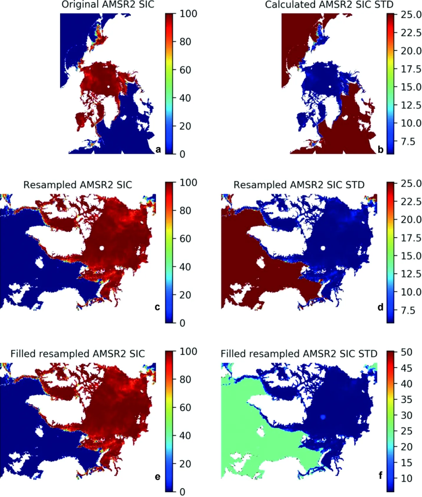
Figure 2 Resampling of 89 GHz AMSR2 SIC and its STD for 20 March 2019: a, Original AMSR2 SIC from University of Bremen; b, Calculated AMSR2 SIC STD using ASI algorithm (Spreen et al., 2008); c, Resampled AMSR2 SIC to the Arctic-20km domain; d, Resampled AMSR2 SIC STD to the Arctic-20km domain; e, Resampled AMSR2 SIC after filling the no-data area; and f, Resampled AMSR2 SIC STD after filling the no-data area. All the units are %.

Compared with the SSMIS SIC, this AMSR2 product has a clear no-data area around the North Pole due to no interpolation made in the original data. This is much clearer in the resampled data on the Arctic-20km domain (Figures 2c and 2d). To fill this missing data area, we again use the interpolation method used for the SSMIS data above. Figures 2e and 2f are the final results after resampling and filling. It is seen that the filled SIC is very smooth and continuous at the North Pole. The extra uncertainty for such filling is again taken a double of the mean STD of the closest 30 grid points. As some of the coastal areas have no data, the interpolated STD in the coastal open water areas becomes double of 0.25.

3.3 Norwegian ice chart

The third product is the ice chart (Figure 3), from Norwegian Ice Service (NIS) at Norwegian Meteorological Institute (Dinessen and Hackett, 2016). The NIS provides daily (working day) ice charts for the European side of the Arctic, covering the east coast of Greenland to the western coasts of Siberia, with the emphasis on Svalbard. The ice chart is produced based on manual interpretation of satellite data, being a typical subjective analysis product. The main satellite data used are the weather independent Synthetic Aperture Radar (SAR) data from RadarSat-2 and Sentinel1. In addition to the SAR data, the analyst uses visual and infrared data from METOP, NOAA and MODIS in cloud free conditions. These satellites data cover the charting area several times a day and are resampled to 1 km grid spacing. The sea ice is classified based on the concentration intervals defined by the WMO (WMO, 1970): fast ice (SIC = 10/10), very closed drift ice (9/10–10/10), closed drift ice (7/10–8/10), open drift ice (4/10–6/10), very open drift ice (1/10–3/10), and open water (0–1/10). The open water here represents sea area of very small amount of ice. For sea area of no ice, we here refer to open sea. As the ice chart only describes SIC with these six classes, for practical use, a mean value is applied to denote the different ice classes in the ice chart. Consequently, these six SIC classes are digitized as 1.0, 0.95, 0.75, 0.5, 0.2 and 0.05, respectively.

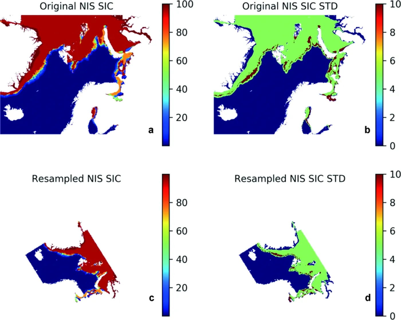
Figure 3 Resampling of NIS SIC and STD for 20 March 2019: a, Original NIS SIC; b, Original NIS SIC STD; c, Resampled SIC to the Arctic-20km domain; and d, Resampled SIC STD to the Arctic-20km domain. All the units are %.

There has been no mature uncertainty analysis so far for the ice chart. In general, the main uncertainty of ice chart comes from the coarse resolution in the SIC space. As only the mean value is used to denote the ice for the whole class, this would cause substantial uncertainties, as the ice in a certain class is not necessary to be its mean, rather it can be any other possible values in the range. In this study, we simply take 0.01 for fast ice, 0.05 for very closed drift ice, closed drift ice and open water, 0.1 for open drift ice and very open drift ice, and 0.0 for open sea, mostly being half of the range of the SIC class. The errors due to the different analysts are not considered here.

3.4 Merging of SIC

As an example, the abovementioned three products are resampled to the Arctic-20km domain, and merged together to the final results (Figure 4). Both SSMIS and AMSR2 products cover the whole Arctic, whereas the ice chart only covers the European side of the Arctic. In general, the SIC difference between SSMIS and AMSR2 is small. However, noticeable difference can be found when SIC is below 50%, particularly at the ice edge, where the AMSR2 SIC appears much sharper. The sharpness of ice edge in the ice chart is generally in between. The open sea region is commonly considered as truly no ice based on the large number of satellite remote sensing observations. In addition, the ice chart has clearer indication for ice-free coastal areas such as the Norwegian and Icelandic coasts, where SSMIS and AMSR2 often produce some ice (Figures 4a and 4c). On the whole, the merged SIC is an improved product containing all the advantages of the three basic products.

The corresponding uncertainties are shown on the right side of Figure 4. There is large difference in the uncertainty fields between SSMIS and AMSR2 (Figures 4b and 4d), although the STD is generally below 0.1 in the ice-covered area. In particular, the SSMIS ice edge is of very high STD up to 0.4 (Figure 4b), whereas in AMSR2 the open water area has high STD up to 0.25 (Figure 4d). In the northern coast of Norway and west coast of Iceland, the SSMIS uncertainty is also high up to 0.4, indicating the difficulties in determining the ice conditions there using coarse- resolution product.

The merged SSMIS+AMSR2 SIC uncertainty is substantially reduced (Figure 4h). In most areas of the Arctic, the STD is below 0.05. At the ice edge, the STD has significantly reduced from the original 0.4 in SSMIS and 0.25 in AMSR2 (Figures 4b and 4d) to about 0.15 (Figure 4h). The ice edge area of high uncertainty is also much narrower compared with the original SSMIS uncertainty (cf. Figures 4b and 4h). The addition of the NIS ice chart further improves the accuracy (cf. Figures 4h and 4j). In the European side of the Arctic, the high uncertainty area is almost fully removed by incorporating the NIS ice chart. However, as the NIS ice chart only covers the European side of the Arctic, some other ice charts such as those from the US National Ice Center, Canadian Ice Service, Danish Ice Service and Russian Ice Service may be further utilized for data merging. This will be investigated in a following study.

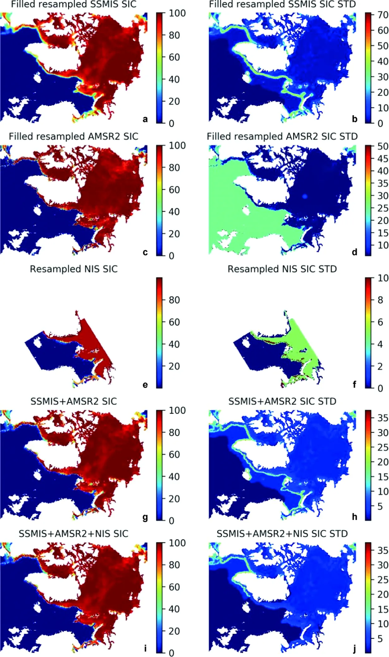
Figure 4 Data merging of SICand STD for 20 March 2019: a, Filled resampled SSMIS SIC; b, Filled resampled SSMIS SIC STD; c, Filled resampled AMSR2 SIC; d, Filled resampled AMSR2 SIC STD; e, Resampled NIS ice chart; f, Resampled SIC STD of NIS ice chart; g, Merged SSMIS+AMSR2 SIC; h, Merged SSMIS+AMSR2 SIC STD; i, Merged SSMIS+AMSR2+NIS SIC; and j, Merged SSMIS+AMSR2+NIS SIC STD. All the units are %.

4 Data merging of SIT products

SIT is a critically important parameter but it is much more difficult to observe through remote sensing. In the present study, we use two products. The first is the daily Soil Moisture and Ocean Salinity (SMOS) SIT from University of Hamburg (Tian-Kunze et al., 2014; Kaleschke et al., 2016), version 3.1, released in October 2016, and now operational. This SMOS SIT was retrieved using surface brightness temperature in L-Band microwave frequency (1.4 GHz) with an iterative retrieval algorithm based on a thermodynamic sea ice model and a three-layer radiative transfer model. The data is gridded at the 12.5 km grid spacing, and is available only from mid-October to mid-April. Figure 5 shows the SMOS SIT and its STD on 20 March 2019. The original SIT and its STD cover a large part of the Arctic sea ice area (Figures 5a and 5b). However, most of these retrieved data are of very high saturation ratio, which contain very high uncertainty in the calculated SIT and STD. According to the data quality description, SMOS SIT data with the STD > 1 m must not be used. For this reason, we remove the SIT and STD data where the STD > 1 m, this resulting in a much smaller area of SIT and SIT STD (Figures 5c and 5d). Such SMOS thin ice has been found of the smallest bias among four different remote sensing products (Wang et al., 2016).

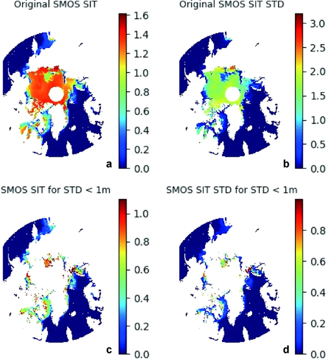
Figure 5 SMOS SIT and its STD on 20 March 2019: a, Original SMOS SIT from University of Hamburg; b, Original SMOS SIT STD from University of Hamburg; c, SIT for STD < 1 m; and d, SIT STD for STD < 1 m. All the units are m.

The second product is the weekly-mean merged CryoSat-2 and SMOS (CS2SMOS) SIT data from Alfred Wegener Institute (Ricker et al., 2017), ftp://ftpsrv2.awi.de/ sea_ice/product/cryosat2_smos/. The data is available from November 2010, also only available in the winter seasons (from October to April). It is a combination of the weekly mean SMOS thin SIT (Tian-Kunze et al., 2014) and the weekly mean CryoSat-2 SIT (Laxon et al., 2013), with the spatially no-data area filled using optimal interpolation method.

The weekly-mean CS2SMOS SIT is not a daily product. In order to achieve the daily estimate, we use a linear interpolation on the time domain by two nearest available datasets. The original weekly-mean CS2SMOS covers a week period, for example, the SIT and STD for 11–17 March 2019 (Figures 6a and 6b), and similarly for 18–24 March 2019 (Figures 6c and 6d). The interpolated daily SIT and STD for 20 March 2019 (Figures 6e and 6f) are linearly interpolated from the above weekly-mean data, which is closer to those on 18–24 March 2019 than those on 11–17 March 2019. Compared with results using weekly data directly, this interpolated daily data shows daily variation rather than no change weekly in the original weekly-mean data.

In this study we merge the daily SMOS SIT and weekly mean CS2SMOS SIT data to form a daily SIT data. Figure 7 illustrated the different products before and after merging for 20 March 2019. The daily SMOS SIT has a very good spatial coverage in the marginal ice zone and coastal region, where SIT is low. The interpolated daily CS2SMOS SIT (Figure 7c) is first filled for the no-data area using the nearest 30 mean to generate the filled daily CS2SMOS SIT (Figure 7e). It is then merged with the daily SMOS SIT, resulting in the merged daily CS2SMOS SIT (Figure 7g), which has a very good spatial coverage for the whole Arctic. This can more clearly be seen from the difference between the merged and the interpolated daily CS2SMOS SIT (Figure 7i), where the merged CS2SMOS SIT improves the data coverage in the coastal areas such as the Canadian Archipelago, Nares Strait and Gulf of Ob. Along the Canadian coast of the Arctic Ocean, the filling also supplements some thick sea ice which was missing in the original weekly mean CS2SMOS SIT.

The corresponding SIT STD is shown on the right side of Figure 7. In general, the STD of the weekly-mean CS2SMOS SIT is between 0.3 m and 0.5 m in the Arctic Ocean, whereas that of the SMOS thin SIT is commonly about 0.2 m. As the SMOS SIT only covers the thin ice part, the merged daily CS2SMOS SIT STD remains largely unchanged compared with the interpolated weekly-mean CS2SMOS SIT. The main improvement of the merged daily SIT STD is the better spatial coverage (Figure 7j), which has a full coverage in the Canadian Archipelago and Ob Bay.

5 Discussion

In this section, we further explore the effect of assimilating the merged data compared with assimilating the original multi-sensor observations, investigate the properties of the error covariance, and examine the assumptions made for the MODM method.

5.1 Assimilation of merged data vs. assimilation of multi-sensor datasets

Assimilation of the merged data or assimilation of the original multi-sensor datasets, which one will generate better results? This is a question we will first explore here. For simplicity, we neglect the whole assimilation loop and focus on the combining of model forecast and observations.We assume the model forecast is already available denoted asf, thus its error vector isf=f−and error covariance= E(ff𝑇). Similar to section 2.1, we again assume the model error vector is random, unbiased and normally distributed, and it is not mutually correlated with the observation error vectors. Thus for model assimilation of the original multi-sensor observations, its optimal estimate f (f;1,2, …,𝑚)can be similarly obtained using the maximum likelihood estimate by minimizing the following cost function,

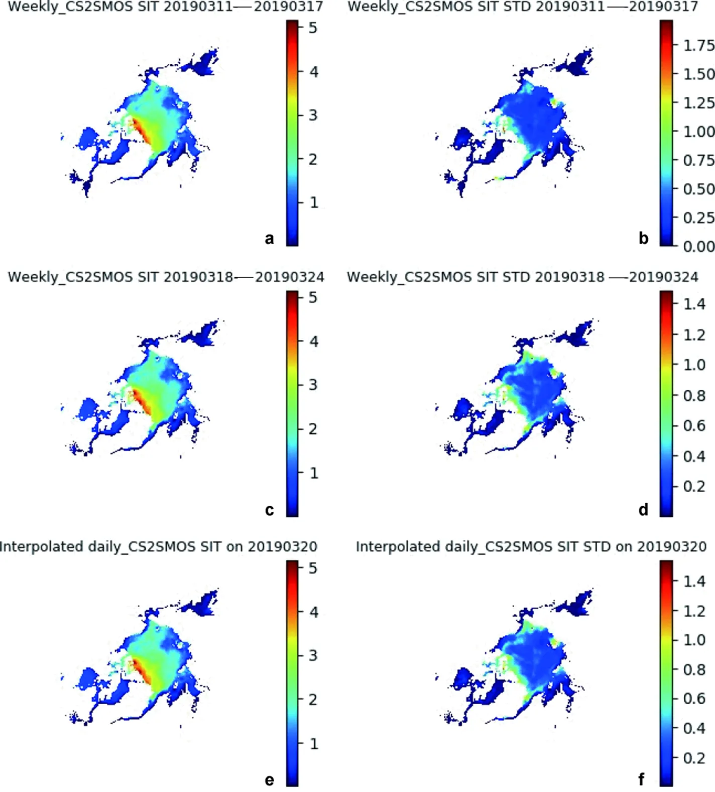
Figure 6 Interpolation of weekly-mean CS2SMOS SIT and its STD for 20 March 2019: a, Original weekly-mean CS2SMOS SIT from 11–17 March 2019; b, Original weekly-mean CS2SMOS SIT STD from 11–17 March 2019; c, Original weekly-mean CS2SMOS SIT from 18–24 March 2019; d, Original weekly-mean CS2SMOS SIT STD from 18–24 March 2019; e, Interpolated daily SIT on 20 March 2019; and f, Interpolated daily SIT STD on 20 March 2019. The data are provided by Alfred Wegener Institute. All the units are m.

This equation is essentially the same as the basic equation for 3DVAR in Caya et al. (2010) and Buehner et al. (2013), except here we have the explicit expression of error covariance for the original multi-sensor observations. Following the same procedure as in section 2.1, we obtain the optimal estimate by assimilating the original multi-sensor observations into the model

where we have used Eqs. (7) and (5a) for simplification. The optimal error vector after data assimilation is therefore

and the corresponding error covariance

Apparently, the optimal estimate(Eq. 12) through direct assimilation of the original multi-sensor observations and its error covarianceP(Eq. 14) are exactly the two-sensor optimal estimate based on model forecastfand error covariancetogether with the merged resultoand error covariance. This indicates that the optimal estimate from assimilation of the merged data is equivalent to the assimilation of the original multi-sensor datasets.

5.2 Properties of error covariance

The covariance of observation error vectors is a central information for merging the multi-sensor datasets. It provides the optimal weights for the concerned data to be involved in the final merged data. Here we explore some of its properties to obtain a deeper understanding of its behavior.

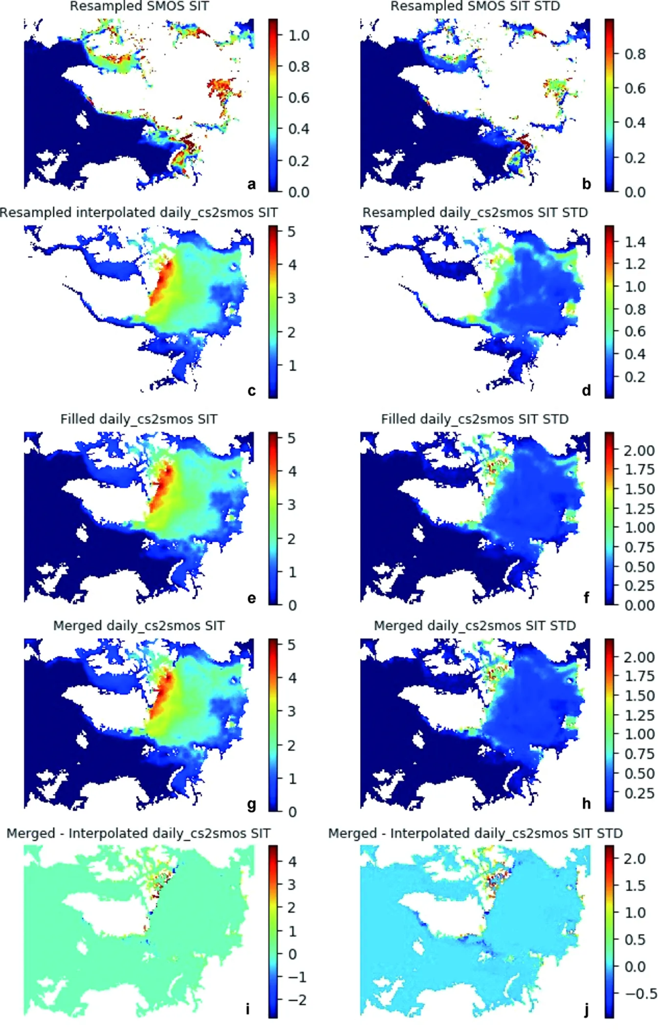
Figure 7 Data merging of SIT and its STD for 20 March 2019: a, Resampled daily SMOS SIT; b, Resampled daily SMOS SIT STD; c, Resampled interpolated daily CS2SMOS SIT for 20 March 2019; d, Resampled interpolated daily CS2SMOS SIT STD for 20 March 2019; e, Filled daily CS2SMOS SIT; f, Filled daily CS2SMOS SIT STD; g, Merged daily CS2SMOS SIT; h, Merged daily CS2SMOS SIT STD; i, Difference between merged daily CS2SMOS SIT and interpolated daily CS2SMOS SIT; and j, Difference between merged daily CS2SMOS SIT STD and interpolated daily CS2SMOS SIT STD. All the units are m.

Denoteas an error vector, thus= E(𝑻) is its covariance. The transpose ofis

Therefore the error covariance is symmetric. In addition, for any real non-zero vector variableof the same length as, we have

where || || denotes the vector norm. Therefore the error covariance is positive semidefinite. Positive semidefinite matrix has only real eigenvalues, all the eigenvalues are non-negative, and its trace equals to the sum of the eigenvalues.

In practice, we often consider the error covariance as positive definite. A positive semidefinite matrix is positive definite if and only if it is nonsingular (Horn and Johnson, 2013). When a positive semidefinite matrix is not positive definite, its determinant is 0. This means some of the rows or columns of the error covariance are linearly dependent on others. In general, we can obtain a positive definite matrix by removing all the linearly dependent rows or columns. As a special positive semidefinite matrix, the positive definite matrix is non-singular and invertible (Horn and Johnson, 2013). It has only real positive eigenvalues, and its trace equals to the sum of the eigenvalues and therefor is also positive. In addition, if we have two positive definite matrices1and2, then1+2is also positive definite. The inversion of1and2, i.e.1−1and2−1, are also positive definite, with their eigenvalues being reciprocal of the eigenvalues of1and2, respectively.

Considered the case for two observations, the merged error covariance (Eq. 7) is

Because1−1and2−1are positive definite,is also positive definite. With simple manipulations of Eq. (17) we get

That is, the trace ofis less than those of both1and2from Eq. (18). For more observations, we can use this method successively. This indicates with more and more observations, the sum of the merged error variance (trace of) will become smaller and smaller, reducing the uncertainty. This can be much more easily seen in the simplified version of Eq. (9). In fact, there have been similar findings from sea ice data assimilation studies, i.e. improving the forecast performance by assimilating more observations (e.g. Caya et al., 2010; Buehner et al., 2013, 2016; Posey et al., 2016; Fritzner et al., 2019).

5.3 Assumptions

In the derivation of MODM, we have made a series of assumptions. The observation error vectors are assumed random, unbiased and normally distributed. These general assumptions are considered as reasonable, and have been widely applied in sea ice data assimilation studies. In fact, if there is a bias in the error vectors and therefore the variable itself, we can remove the bias by subtracting the identified bias. While SIC is absolutely not normally distributed, its error vector may be considered as normally distributed. This is particularly true for remote sensing: when some radiative signal levels are defined for the cases of SIC = 1 or SIC = 0, there are still higher- or lower-level radiative signals exist in the dataset (e.g. Spreen et al., 2008; Lavergne et al., 2019). Therefore, a normal distribution of the error vector can be reasonable at least in remote sensing.

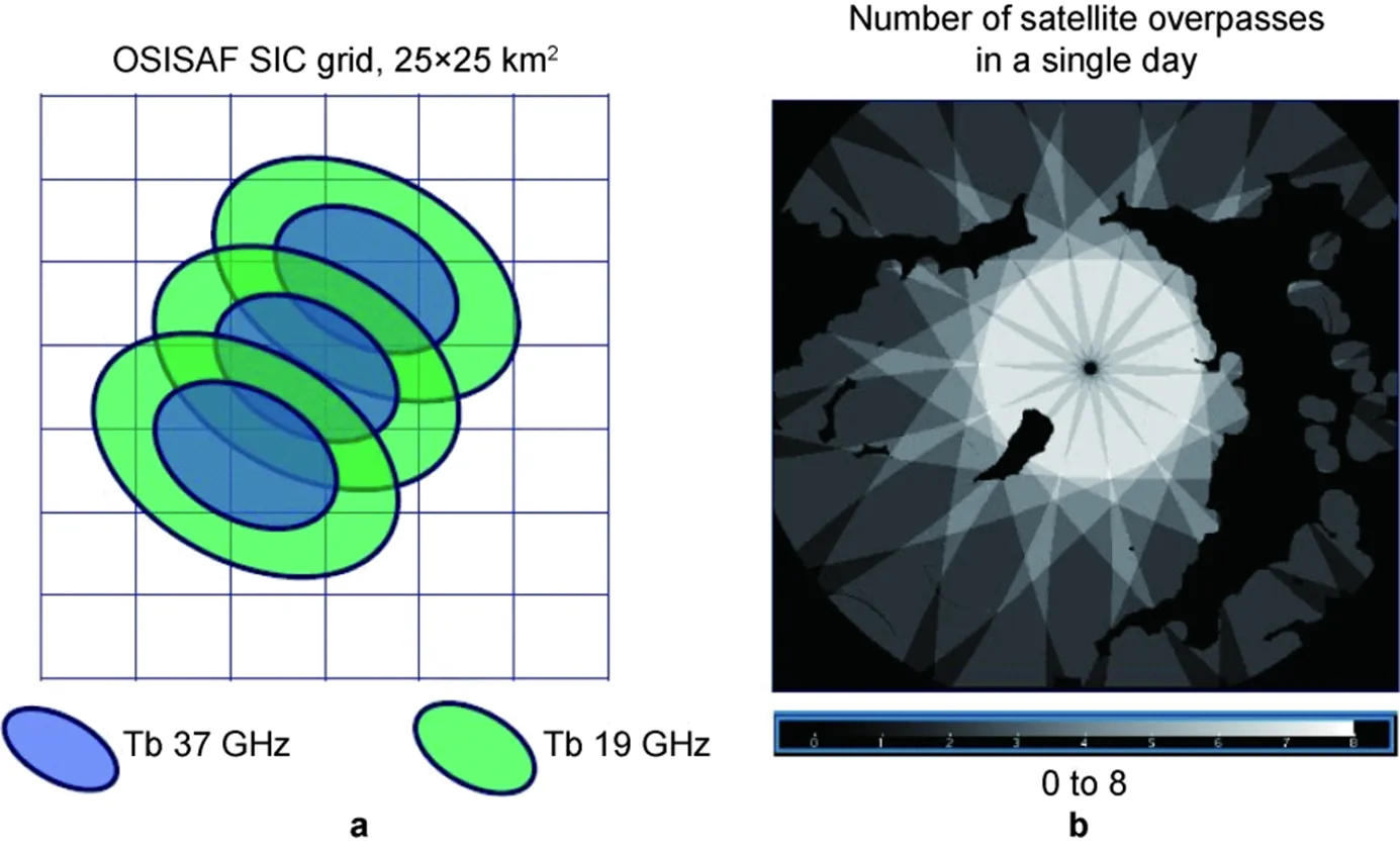
Figure 8 a, Footprints of Tb 37 GHz and Tb 19 GHz on the OSISAF SIC 25km-grid; b, Number of satellite overpasses in a single day.

In the application part using the simplified version of MODM, we have assumed no spatial correlation in each individual error vectors. This assumption significantly facilitate the calculation, however, it may be not well-satisfied. Figure 8a show the footprints of the Tb 37 GHz and Tb 19 GHz on the OSISAF SIC grid. It is seen that their footprints are larger than the output grid. Thus, a single SIC observation contributes to several grid cells. This leads to the spatial correlation of the uncertainties. If we further compare the uncertainty distribution (Figure 1b) with the number of satellite overpasses in a single day (Figure 8b), there is no imprint of observation number on the uncertainty map. This indicates that the uncertainty does not scale to the reciprocal of square root of the observation number, which again suggests the possible spatial correlation of the uncertainties. Daley (1991) analyzed multiple-observation problem for atmospheric data. While he considered spatial correlation in the background field, his analysis was also based on the presumption that the multiple-observation errors are spatially uncorrelated. In the present study, with the basic equations (Eqs. 5 and 7) and observed spatial correlations, the MODM method provide one feasible way to the optimal estimate for multiple spatially correlated observation vectors. An alternative solution may be to use higher resolution products, so that we can still use the simplified method (Eqs. 9 and 10). In this sense, the 89 GHz AMRS2 SIC does provide a good basis for optimal estimate of spatially uncorrelated observations.

When deducing the compact error covariance (Eq. 7), we have assumed that different observation error vectors are not mutually correlated. This may not always be the case, because most datasets will try to use multiple data sources to improve the quality. For example, in the current study the sea ice chart is already an objectively merged product using a large number of remote sensing products. The merged daily SIT here uses a daily SMOS SIT together with two neighboring weekly-mean CS2SMOS SIT. Since the weekly-mean CS2SMOS SIT already uses SMOS SIT, the SMOS SIT and the weekly-mean CS2SMOS SIT are somewhat correlated in the thin ice area. For this case, we may estimate the extra error variance for the merged daily SIT uncertainty. Following the same procedure as Eq. (7) and assume that all the other assumptions still applies, we can see the final result will be 9/7 of the current error variance, i.e. about 13% more than the current standard deviation. The change in the error variance will generally affect the optimal estimateo. However, in the present study it is basically a replacement of the weekly-mean SMOS SIT by daily SMOS SIT. Such a replacement is obviously more consistent with the daily data requirement.

6 Concluding remarks

Due to the increasing interest in the polar region and the development of new satellite technologies, a large number of sea ice remote sensing data have been generated in recent years, and it is expected that such increasing will continue in the near future. In order to make the best use of such large number of datasets, a statistically based MODM method is introduced to merge an arbitrary large number of observations, calculating the optimal estimate and uncertainty. It is assumed that all the observation error vectors are random, unbiased and normally distributed, and that any two of the observation vectors should be not mutually correlated. For practical applications, a simplified version of MODF is deduced, assuming no spatial correlation in any observation error vector. This assumption is made to fit the current satellite sea ice remote sensing products, in which only local standard deviation is provided (e.g. Tian-Kunze et al., 2014; Dinessen and Hackett., 2016; Ricker et al., 2017; Lavergne et al., 2019). When the full estimate of error covariance is available, we can use the general equations (Eqs. 5 and 7) to merge different observations.

One important advantage of the MODM method is to provide a complete optimal estimate of the concerned field and its uncertainties purely through observations. So it can be used not only for better real-time monitoring, but also for model initialization and model validation. In addition, we have shown that assimilation of the merged data is equivalent to assimilate the original multi-sensor datasets. This greatly facilitates the data assimilation procedure, as we may use a large variety of assimilation methods, which will provide similar assimilation and forecast quality regardless of using 3DVAR, direct insertion, nudging, or ensemble Kalman filter when assimilating the same sea ice observations (e.g. Caya et al., 2010; Fritzner et al., 2018).

We have applied the simplified MODM method for optimal estimate of SIC and SIT products in this study. The results show that the MODM has high capability in reducing the observation uncertainties and increasing the spatial coverage of the data. From the merging of SIC, the MODM improved the ice edge and removed the fake ice along the Norwegian and Icelandic coasts. Due to the limited datasets in the current study, the merged SIC STD still has further potential to improve, particularly for Davis Strait, Baffin Bay and Southern Greenland coast. Additional ice charts from Canadian Ice Service and Danish Ice Service would be very beneficial to such improvement. For the merging of SIT, we see that the merged daily CS2SMOS SIT has a substantial improvement compared with the pure daily SMOS SIT. It also has a marked improvement compared with the weekly-mean CS2SMOS SIT, as it has a closer thin SIT to the daily SMOS SIT than the weekly-mean CS2SMOS SIT. It also provides a better spatial coverage of SIT for the coastal areas and bays.

In the discussion of the error covariance, we have shown that the uncertainties of the merged data are always not large than any of the original observations. The MODM tends to maintain the best observed data (lowest uncertainty), and neglect the high-uncertainty data. This can be clearly seen in the SIT merging (Figure 7). For most thick ice area, the merged SIT remains unchanged compared with the original data. For the thin ice area, it is the daily SMOS SIT that replaced the weekly-mean SMOS SIT. In this case, the improvement due to the MODM is apparent for daily purpose. It is noteworthy that, as a statistical method, the optimal solution of MODM depends strongly on the data quality of the original multi-sensor data. It is particularly important to avoid mismarking the erroneous data as low-uncertainty data, which may deteriorate the overall optimal estimate.

Acknowledgments EUMETSAT, Norwegian Ice Service, University of Bremen, University of Hamburg, and Alfred Wegener Institute are gratefully acknowledged for providing the data. We thank two anonymous reviewers for their helpful comments. This study was supported by the Norwegian Research Council through the SPARSE project (Grant no. 254765) and CIRFA project (Grant no. 237906).

Buehner M, Caya A, Pogson L, et al. 2013. A new environment Canada regional ice analysis system. Atmosphere-Ocean, 51(1): 18-34, doi: 10.1080/07055900.2012.747171.

Buehner M, Caya A, Carrieres T, et al. 2016. Assimilation of SSMIS and ASCAT data and the replacement of highly uncertain estimates in the Environment Canada Regional Ice Prediction System. QJR Meteorol Soc, 142(695): 562-573, doi: 10.1002/qj.2408.

Caya A, Buehner M, Carrieres T. 2010. Analysis and forecasting of sea ice conditions with three-dimensional variational data assimilation and a coupled ice–ocean model. J Atmos Oceanic Technol, 27(2): 353-369, doi: 10.1175/2009jtecho701.1.

Daley R. 1991. Atmospheric data analysis (Cambridge atmospheric and space science series). Cambridge: Cambridge University Press.

Dinessen F, Hackett B. 2016. Product user manual for regional high resolution sea ice charts Svalbard region, PUM for Sea Ice TAC regional Arctic sea ice product. SEAICE_ARC_SEAICE_L4_ NRT_OBSERVATIONS_011_002, Issue: 2.7, 15 January 2018. http://marine.copernicus.eu/documents/PUM/CMEMS-OSI-PUM-011-002.pdf.

Fritzner S M, Graversen R G, Wang K G, et al. 2018. Comparison between a multi-variate nudging method and the ensemble Kalman filter for sea-ice data assimilation. J Glaciol, 64(245): 387-396, doi: 10.1017/jog.2018.33.

Fritzner S, Graversen R, Christensen K H, et al. 2019. Impact of assimilating sea ice concentration, sea ice thickness and snow depth in a coupled ocean–sea ice modelling system. Cryosphere, 13(2): 491-509, doi: 10.5194/tc-13-491-2019.

Horn R A, Johnson C R. 2013. Matrix analysis. Cambridge: Cambridge University Press, 431.

IPCC. 2014. Climate change 2014: synthesis report. Contribution of Working Groups I, II and III to the fifth assessment report of the Intergovernmental Panel on Climate Change//Core Writing Team, Pachauri R K, Meyer L A. IPCC, Geneva, Switzerland, 151.

Kaleschke L, Tian-Kunze X, Maaß N, et al. 2016. SMOS sea ice product: Operational application and validation in the Barents Sea marginal ice zone. Remote Sens Environ, 180: 264-273, doi: 10.1016/j.rse.2016.03. 009.

Kalnay E, Li H, Miyoshi T, et al. 4-D-Var or ensemble Kalman filter? Tellus A, 2007, 59(5): 758-773.

Lavergne T, Sørensen A M, Kern S, et al. 2019. Version 2 of the EUMETSAT OSI SAF and ESA CCI sea-ice concentration climate data records. Cryosphere, 13(1): 49-78, doi: 10.5194/tc-13-492019.

Laxon S W, Giles K A, Ridout A L, et al. 2013. CryoSat-2 estimates of Arctic sea ice thickness and volume. Geophys Res Lett, 40(4): 732-737, doi: 10.1002/grl.50193.

Lindsay R W, Zhang J. 2006. Assimilation of ice concentration in an ice–ocean model. J Atmos Oceanic Technol, 23(5): 742-749, doi: 10.1175/jtech1871.1.

Lisæter K A, Rosanova J, Evensen G. 2003. Assimilation of ice concentration in a coupled ice—ocean model, using the Ensemble Kalman filter. Ocean Dyn, 53(4): 368-388, doi: 10.1007/s10236-003- 0049-4.

Melsheimer C. 2019. ASI Version 5 Sea Ice Concentration User Guide, Version V0.92 (August 4, 2019). University of Bremen.

Posey P G, Metzger E J, Wallcraft A J, et al. 2015. Improving Arctic sea ice edge forecasts by assimilating high horizontal resolution sea ice concentration data into the US Navy’s ice forecast systems. Cryosphere, 9: 1735-1745, doi: 10.5194/tc-9-1735-2015.

Ricker R, Hendricks S, Kaleschke L, et al. 2017. A weekly Arctic sea-ice thickness data record from merged CryoSat-2 and SMOS satellite data. Cryosphere, 11(4): 1607-1623, doi: 10.5194/tc-11-1607-2017.

Sakov P, Counillon F, Bertino L, et al. 2012. TOPAZ4: an ocean-sea ice data assimilation system for the North Atlantic and Arctic. Ocean Sci, 8(4): 633-656, doi: 10.5194/os-8-633-2012.

Spreen G, Kaleschke L, Heygster G. 2008. Sea ice remote sensing using AMSR-E 89-GHz channels. J Geophys Res-Oceans, 113(C2): C02S03, doi: 10.1029/2005jc003384.

Stark J D, Ridley J, Martin M, et al. 2008. Sea ice concentration and motion assimilation in a sea ice–ocean model. J Geophys Res-Oceans, 113(C5): C05S91, doi: 10.1029/2007jc004224.

Tian-Kunze X, Kaleschke L, Maaß N, et al. 2014. SMOS-derived thin sea ice thickness: algorithm baseline, product specifications and initial verification. Cryosphere, 8(3): 997-1018, doi: 10.5194/tc-8-997-2014.

Tietsche S, Notz D, Jungclaus J H, et al. 2013. Assimilation of sea-ice concentration in a global climate model–physical and statistical aspects. Ocean Sci, 9: 19-36, doi: 10.5194/os-9-19-2013.

Todling R. 1999. Estimation theory and foundations of atmospheric data assimilation. DAO Office Note 1999-01.

Tonboe R T, Eastwood S, Lavergne T, et al. 2016. The EUMETSAT sea ice concentration climate data record. Cryosphere, 10(5): 2275-2290, doi: 10.5194/tc-10-2275-2016.

Wang K G, Debernard J, Sperrevik A K, et al. 2013. A combined optimal interpolation and nudging scheme to assimilate OSISAF sea-ice concentration into ROMS. Ann Glaciol, 54(62): 8-12, doi: 10.3189/2013aog62a138.

Waters J, Lea D J, Martin M J, et al. 2015. Implementing a variational data assimilation system in an operational 1/4 degree global ocean model. QJR Meteorol Soc, 141(687): 333-349, doi: 10.1002/qj.2388.

World Meteorological Organization (WMO). 1970. WMO sea-ice nomenclature: terminology, codes, illustrated glossary and symbols. Geneva: Secretariat of the World Meteorological Organization. 145.

Yang Q H, Losa S N, Losch M, et al. 2014. Assimilating SMOS sea ice thickness into a coupled ice-ocean model using a local SEIK filter. J Geophys Res-Oceans, 119(10): 6680-6692, doi: 10.1002/2014jc 009963.

Zhang J L, Thomas D R, Rothrock D A, et al. 2003. Assimilation of ice motion observations and comparisons with submarine ice thickness data. J Geophys Res-Oceans, 108(C6): 3170, doi: 10.1029/2001jc 001041.

12 March 2019;

12 December 2019;

6 March 2020

: Wang K G, Lavergne T, Dinessen F. Multi-sensor data merging of sea ice concentration and thickness. Adv Polar Sci, 2020, 31(1): 1-13,

10.13679/j.advps.2019.0016

, E-mail: Keguang.wang@met.no

10.13679/j.advps.2019.0016