Features of sea ice motion observed with ice buoys from the central Arctic Ocean to Fram Strait

HAN Hongwei, LEI Ruibo, LU Peng & LI Zhijun

Features of sea ice motion observed with ice buoys from the central Arctic Ocean to Fram Strait

HAN Hongwei1, LEI Ruibo2*, LU Peng3& LI Zhijun3

1School of Water Conservancy and Civil Engineering, Northeast Agricultural University, Harbin 150030, China;2MNRKey Laboratory for Polar Science, Polar Research Institute of China, Shanghai 200136, China;3Laboratory of Coastal and Offshore Engineering, Dalian University of Technology, Dalian 116024, China

Using six ice-tethered buoys deployed in 2012, we analyzed sea ice motion in the central Arctic Ocean and Fram Strait. The two-hourly buoy-derived ice velocities had a magnitude range of 0.01–0.80 m·s−1, although ice velocities within the Arctic Basin were generally less than 0.4 m·s−1. Complex Fourier transformation showed that the amplitudes of the sea ice velocities had a non-symmetric inertial oscillation. These inertial oscillations were characterized by a strong peak at a frequency of approximately −2 cycle·d−1on the Fourier velocity spectrum. Wind was a main driving force for ice motion, characterized by a linear relationship between ice velocity and 10-m wind speed. Typically, the ice velocity was about 1.4% of the 10-m wind speed. Our analysis of ice velocity and skin temperature showed that ice velocity increased by nearly 2% with each 10 ℃ increase in skin temperature. This was likely related to weakened ice strength under increasing temperature. The ice-wind turning angle was also correlated with 10-m wind speed and skin temperature. When the wind speed was less than 12 m·s−1or skin temperature was less than −30 ℃, the ice-wind turning angle decreased with either increasing wind speed or skin temperature. Clearly, sea ice drift in the central Arctic Ocean and Fram Strait is dependent upon seasonal changes in both temperature and wind speed.

Arctic sea ice, velocity, inertial oscillation, wind, skin temperature

1 Introduction

Arctic sea ice as a sensitive indicator of global climate change has undergone dramatic changes over the past few decades. In September 2012, the extent of the Arctic sea ice was the lowest recorded by satellite observations since 1979 (Zhang et al., 2012). The ongoing decline in Arctic sea ice extent has been attributed to increases in surface air temperature and ocean heat storage (Polyakov et al., 2010). Under conditions of global warming, polar amplification produces a larger than average change in temperature near the poles (Lee, 2014). This has resulted in Arctic surface air temperatures increasing twice as much as the global average in recent decades (Gao et al., 2015). Arctic warming has accelerated the melting of Arctic sea ice, causing a decrease in ice extent, ice thickness and the length of the ice season (Vihma, 2014). From 1979 to 2010, satellite data documented a decreases in Arctic sea ice extent of −12.2%·(10 a)–1(Comiso, 2012), with a mean monthly ice volume anomaly of −2.8 × 103km3·(10 a)–1from 1979 to 2010 (Schweiger et al., 2011). This decline in Arctic ice volume is associated with a 37% decrease in ice mechanical strength and 31% decrease in ice internal force during the period 2007–2011, compared to mean values for 1979–2006 (Zhang et al., 2012). It has also led to increasing ice drift, as the ice becomes thinner. A correlation between drift speed and ice concentration has occurred, as ice more readily responds to synoptic-scale forcing of the atmosphere (Olason and Notz, 2014).

The method of observing sea ice motion includesLagrangian drifters as well as satellite-acquired images from optical, thermal, radar and passive-microwave instruments (Heil et al., 2001). Buoy data are most accurate and have small measurement errors, while satellite data are able to cover the sea ice zone more effectively (Zhang et al., 2003). The International Arctic Buoy Programme (IABP; http://iabp.apl.washington.edu/) has collected and archived position data of ice-tethered buoys deployed in the Arctic Ocean since 1979. Since the 1990’s, these satellite data have provided a unique monitoring capability of sea ice drift measurements over the Arctic and Antarctic (Martin and Augstein, 2000). UsingLagrangian drifters, we can study the dynamics of sea ice to determine the state of sea ice cover as well as its climatic and oceanic interactions. They can also be used to evaluate sea ice mass balances and to precisely track the source and fate of sea ice.

Sea ice drifts, deforms, and fractures under external forces, essentially wind and ocean stresses, subject to its boundaries (Weiss, 2013). As the Arctic ice cover thins, it becomes more susceptible to wind forcing. Ogi and Rigor (2013) suggested that winter westerly winds over the Beaufort Sea and summer anticyclonic circulation over the Arctic towards the Fram Strait have contributed to accelerated decreases in sea ice in areas east of Europe and north of Alaska in recent years. This strong anticyclonic circulation has also caused more rapid decreases in the Arctic sea ice during summer periods since 1996. Several previous studies (Kwok, 2000; Zhao and Liu, 2007; Vihma et al., 2012) have indicated that sea ice motion occurs in response to the dominant pattern of atmospheric circulation, including the Arctic/North Atlantic Oscillation (AO/NAO), and Pacific Decadal Oscillation (PDO). Based on IABP data (1979–1998), Rigor et al. (2002) found that high-index conditions of the wintertime Arctic Oscillation (AO) reduced Arctic sea ice by enhancing production of thin ice located away from coastal regions, while increasing ice advection out of the Arctic through the Fram Strait. Maslanik et al. (2007) found that wind and ice transport patterns have favored reduced ice cover in the western and central Arctic since the late 1980s, but that the AO index was not a reliable indicator of these patterns.

We studied sea ice motion within the central Arctic Ocean and Fram Strait, using data collected by six ice-tethered buoys. In section 2, we briefly present the data and methods used in this study; while in section 3, we present our analysis of sea ice velocity, inertial oscillation, and the ice drift response to surface wind and air temperature. Lastly, we summarize the conclusions of our study.

2 Data and methods

The buoys deployed during 2012 are shown in Table 1. They consisted of five Sea Ice Measurement Balance Arrays (SIMBA; Scottish Association for Marine Science, Scotland; buoys A–E), and one Ice Mass Balance buoy (IMB; MetOcean, Canada; buoy F). The ice mass balance processes measured by these buoys were characterized by Lei et al. (2018).

After their deployment, driven by the Transpolar Drift Stream (TDS), three buoys (buoys C, D and F) drifted from the central Arctic Ocean into the Fram Strait over a period of 7−11 months (Figure 1). The other three buoys (buoys A, B and E) remained within the central Arctic Ocean over their short operational lifetimes.

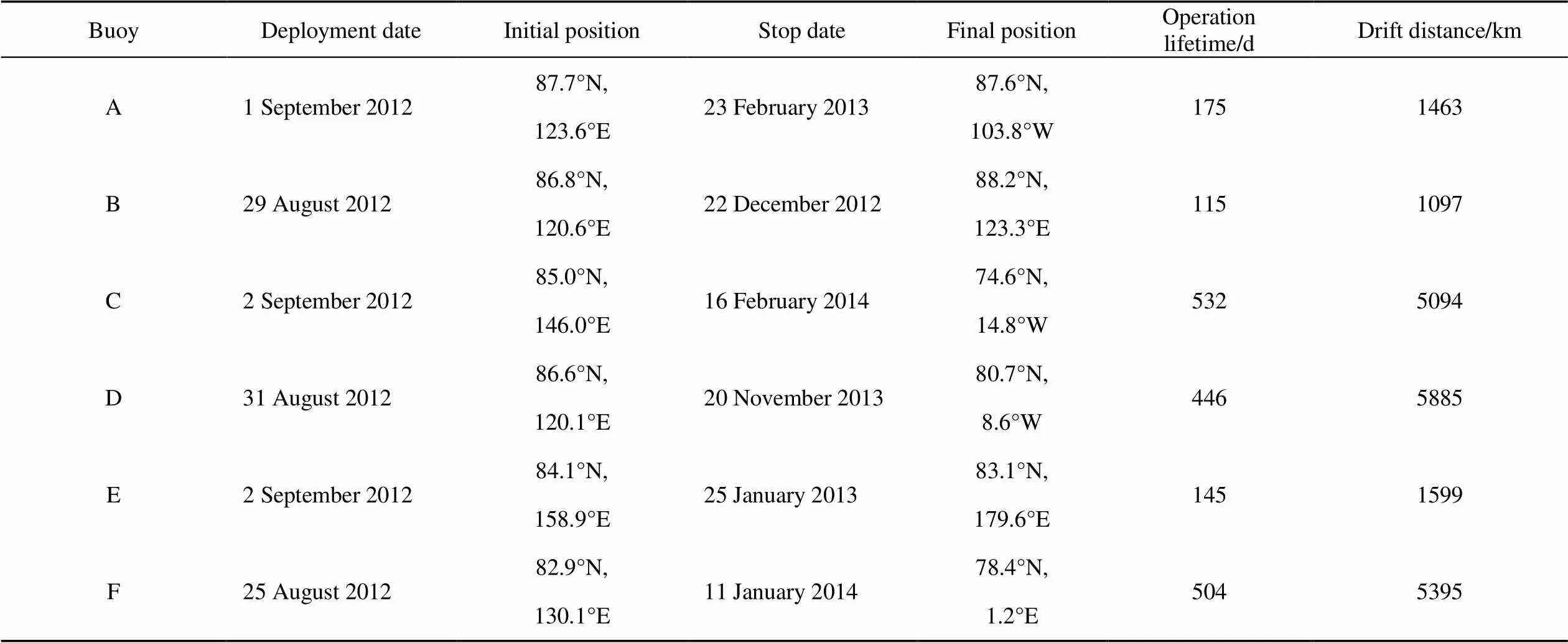
Table 1 Operational history of the six buoys deployed in the central Artic Ocean in 2012

Figure 1 Trajectories of the six buoys (A–F) deployed in 2012 in the central Artic Ocean.

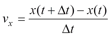
The raw buoy positions were linearly interpolated to the same temporal interval (2 h), before calculating ice drift velocity data. The sea ice velocity was calculated from successive positions, using:

According to Leppäranta (2011), the accuracyδof the ice velocity is calculated using:

whereis the number of velocity samples along the buoy trajectory and= 2πis the angular frequency. This Fourier transformation distinguishes negative and positive frequencies associated with clockwise and anticlockwise oscillations, respectively.

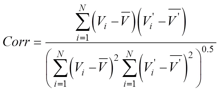
Sea ice concentrations were derived from the daily Advanced Microwave Scanning Radiometer-2 data (http://www.iup.uni-bremen.de:8084/amsr2/). We used six- hourly derived 10-m wind speed and skin temperature data with a horizontal resolution of 2.5° (latitude and longitude) from the National Centers for Environmental Prediction (NCEP)/Department of Energy (DOE) Reanalysis 2 data, available at http://www.esrl.noaa.gov/psd/(Kanamitsu et al., 2002), to ascertain the local atmospheric forcing along the buoy’s trajectory. Processing errors are unavoidable in these reanalysis data, resulting in some differences between predicted and real data. These data flaws are not considered herein. The skin temperature and 10-m wind speed data were integrated with the vector field of buoy trajectory at the same scale, using linear interpolation of space and time of the NCEP/DOE Reanalysis 2 data. The ice drift direction was classified using the absolute value of the turning angle between the ice drift and the wind vector, according to Vihma et al. (1996). Ice-wind turning angles of less than 45° were assigned to “with wind heading”; while angles between 45° and 135° were assigned to “perpendicular to wind heading”; and angles larger than 135° to “against wind heading”. The correlation coefficient between the sea ice drift and wind speed was calculated using:

3 Results

3.1 Sea ice velocity

Figure 2 presents the hourly v(zonal ice speed) andv(meridional ice speed) at buoys A and C. The mean values ofvandvat buoy C were larger than those at buoy A, while the standard deviations ofvandvat both buoys had similar values. As buoy C drifted through the Fram Strait, the ice speed increased rapidly, especially its meridional ice speed. This caused buoy C to have a high dispersion in meridional ice speed, yielding a larger standard deviation.

As shown in Figure 3, the magnitude of the two-hourly buoy-derived ice velocity ranged from 0.01 to 0.80 m·s−1. In contrast, the ice velocities of buoys A, B and E drifting within the Arctic Basin were generally less than 0.40 m·s−1. Before buoys C, D and F drifted into the Fram Strait, their ice velocities were also generally less than 0.40 m·s−1. All velocities were substantially greater than the average ice velocity of 0.077 m·s−1observed for the entire Arctic Ocean during 1976–2006, and that of 0.078 m·s−1observed during 2007–2011 (Zhang et al., 2012). This is partly because these buoys were deployed in the TDS region, where ice velocities are typically higher. A previous study revealed that the average ice velocity of the Arctic Ocean shows strong seasonal changes, with a maximum in October and a minimum in April (Rampal et al., 2009). The ice velocity probability distribution was acquired every month at buoys C, D and F from September 2012 to December 2013 at intervals of 0.01 m·s−1. The probability distribution of ice speed exhibited a significant monthly change (Figure 4). Concurrently, the ice velocity probability distributions of these three buoys showed self-similarity every month. Before buoys C, D and F drifted into the Fram Strait, the ice velocity probability distribution was concentrated in February, April and July of 2012, with ice velocities of less than 0.2 m·s−1. In September, October and November of 2012, ice velocities greater than 0.2 m·s−1increased markedly, causing a more dispersed probability distribution. As buoys C and F drifted southward into the range of 79°N–85°N (into the Fram Strait), the ice velocity probability distribution became extremely dispersed (November and December 2013). This is consistent with the previous finding that ice velocity increased, as the sea ice moved into the Fram Strait.

Figure 2 Scatterplot of hourly v(zonal ice speed) andv(meridional ice speed) at buoys A and C. Subpanels show the probability (blue line) with a bin width of 0.02 m·s−1and normal distribution probability density (red line) for these speeds.

Figure 3 Variations in two-hourly buoy-derived ice velocities over the entire drifting period for all the six buoys (A–F) deployed in 2012.

3.2 Inertial oscillation

Under the Coriolis force, the Arctic sea ice moves in a circular orbit, referred to as an inertial oscillation. Unlike semi-diurnal tidal oscillations that can cause circular orbits in both clockwise and anticlockwise directions, wind- generated inertial oscillations only rotate in a clockwise direction in the northern hemisphere (Stoudt, 2015). The frequency of this inertial oscillation depends on the latitude; it can be calculated using:

Figure 4 Ice velocity distributions represented as percentages each month at buoys C, D and F from September 2012 to December 2013. The white areas indicate no data were available in the corresponding velocity bins.

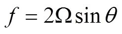
whereis the inertial frequency in units of cycle·d−1,Wis the Earth rotation rate (1.002736 cycle·d−1) andis the latitude. The six buoys were distributed in a defined area (between 82°N and 89°N within the Arctic Basin) in October 2012. At this time, their inertial oscillation frequencies varied from −1.986 to −2.005 cycle·d−1. Complex Fourier transformation shows that the amplitudes of the sea ice velocity had non-symmetric inertial oscillations at all the six buoys. The peak at= 0 represents the advective component of the buoy motion, while inertial oscillations are defined by a strong peak observed at a frequency of approximately −2 cycle·d−1on the Fourier velocity spectrum, which is close to the value determined from theoretical calculation (Figure 5). The amplitudes of the semi-diurnal frequencies showed marked differences among the six buoys. After Fourier transformation, the amplitudes of the semi-diurnal frequencies at the buoys C, E and F were higher than those at buoys A, B and D. Inertial oscillations can be related to ice concentration and internal stress. Although sea ice concentrations were greater than 90% in October 2012 (Figure 6), the inertially induced ice movement (damped by internal stress) decreased as the buoys drifted into the marginal ice zone. This likely explains why the amplitude of the semi-diurnal frequency at buoy F was higher than that of all other buoys.

3.3 Response to surface wind forcing

The monthly distributions of both wind headings and ice vectors at buoy C in 2013 are shown in Figure 7. The ice vectors remained east of the wind direction over the range of 20°–30°. This is consistent with the deviated force of the Earth’s rotation in the northern hemisphere (positive rotation).The buoy C drifted into the Fram Strait in December 2013. In this month, the dominant wind heading ranged from northwest to northeast, coincident with the TDS. This caused the buoy to drift through the Fram Strait in less than a month. Figure 8 shows the probability of the turning angle between the ice drift and the wind vector at buoy C in 2013. Generally, the probability of “against wind heading” each month was less than 9%. In contrast, a minimum probability of “with wind heading” of 37% occurred during the summer (June, July and August), while in other seasons it was mostly greater than 60%.

There is a clear linear relationship between the observed ice velocity and 10-m wind speed shown in Figure 9, in which the ice velocity is typically about 1.4% of the 10-m wind speed. This is slightly smaller than the rule-of-thumb, suggesting that sea ice speed is about 2% of the surface wind speed (Thorndike and Colony, 1982). When the 10-m wind speed was less than 13 m·s−1, the positive linear relationship improved between the observed ice velocity and 10-m wind speed. Once 10-m wind speed exceeded 13 m·s−1, the ice velocity fluctuated greatly, as it increased. This is because at higher of wind speed more uncertainties are introduced, related to the increase in interactions among the ice floes. Usually, wind is the driving force of ice motion, but at low wind speed, wind plays a less important role. When the 10-m wind speed was less than 3 m·s−1, there was no clear relationship between ice motion and wind speed (Figure 10). The ratio of ice speed to the 10-m wind speed was within the range of 0.01–0.02, when wind speeds were larger than 3 m·s−1. Under free drift conditions, Leppäranta (2011) showed that the wind caused a rapid decrease in ice speed, when wind speed was within the range of 3–4 m·s−1.

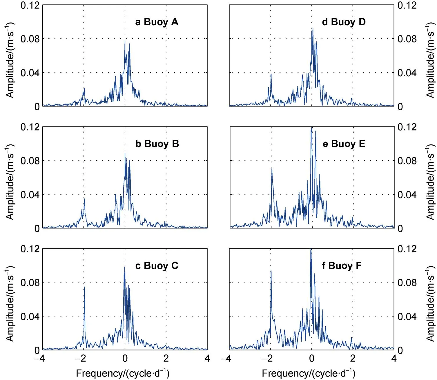
Figure 5 Amplitudes after Fourier transformation of the sea ice velocity vector for all six buoys (A–F) in October 2012.

Figure 6 Monthly sea ice concentration for October 2012. The trajectories of all six buoys (A–F) are denoted by white lines.

In addition to the linear relationship between ice velocity and wind speed, there are seasonal changes in the response of ice velocity to wind speed. Figure 11 shows the monthly correlation coefficients between ice velocity and wind speed at buoys C, D and F. These results show that the correlation coefficients for all three buoys during the first two months (December 2012 and January 2013) of winter were greater than or equal to 0.8; while in July, August and September 2013, the correlation coefficients were less than 0.7. The sea ice surface morphology dramatically changes as the sea ice thickness and ice concentration decrease in summer. In particular, the surface roughness decreases as the sea ice melts. Such changes were associated with enhanced inertial motion as summer approached, weakening the effect of wind forcing on the sea ice.

Figure 7 Monthly distributions (%, scaled by total measurements given in magenta) of wind headings (blue) and ice vectors (red) at buoy C in 2013. The latitude interval is given in square brackets in each panel.

Figure 8 Probability of various ice-wind turning angles between the ice drift and the wind vector at buoy C in 2013. Angles within 45° of the wind direction were assigned to “with wind heading”; angles between 45° and 135° to “perpendicular to wind heading”; and angles greater than 135° to “against wind heading”.

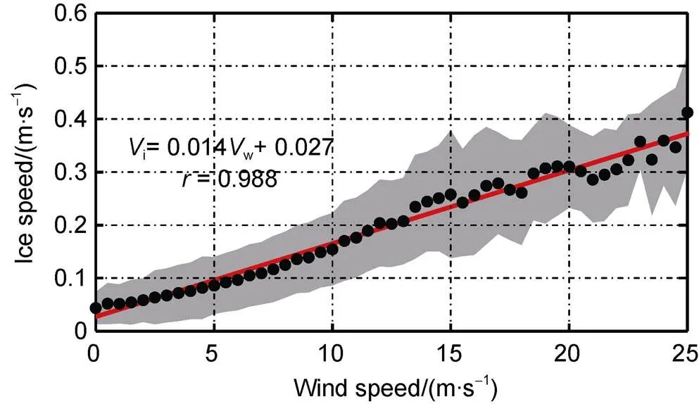
Figure 9 Relationship between ice velocity and 10-m wind speed. The black dots show the mean ice velocity calculated from all buoy data, while the gray shading indicates one standard deviation from the mean. The red line shows the linear regression line.

Figure 10 Ratio of ice speed to 10-m wind speed. The black dots show the mean ratio calculated from all buoy data, while the gray shading indicates one standard deviation from the mean.

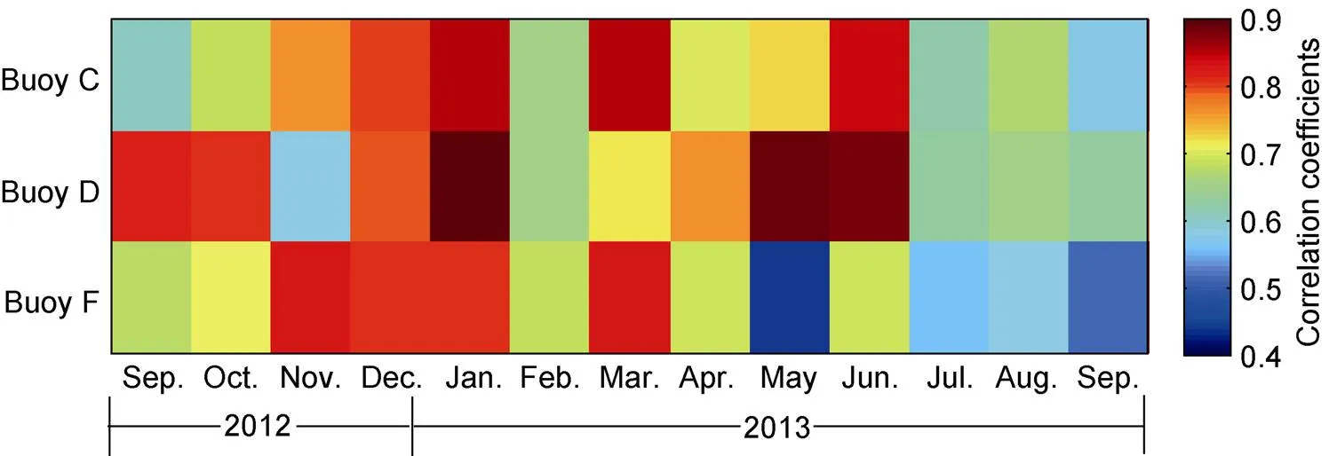
Figure 11 Monthly correlation coefficients between ice velocity and 10-m wind speed at buoys C, D and F from September 2012 to September 2013.

The ice-wind turning angle is another parameter used to describe the relationship between ice drift and wind direction. The ice-wind turning angle is generally defined as positive, when the ice drift is to the east of the wind in the northern hemisphere. Figure 12 shows the ice-wind turning angle decreased with increasing 10-m wind speed. This is consistent with results of previous studies (Thorndike and Colony, 1982; Park and Stewart, 2015). When the 10-m wind speed was less than 12 m·s−1, the ice-wind turning angle decreased with increasing wind velocity, reaching a maximum of 87° when the wind speed was close to zero. The standard deviation of the ice-wind turning angle also increased as wind speed decreased. Once 10-m wind speeds exceeded 12 m·s−1, the ice-wind turning angle stabilized to around 30°.

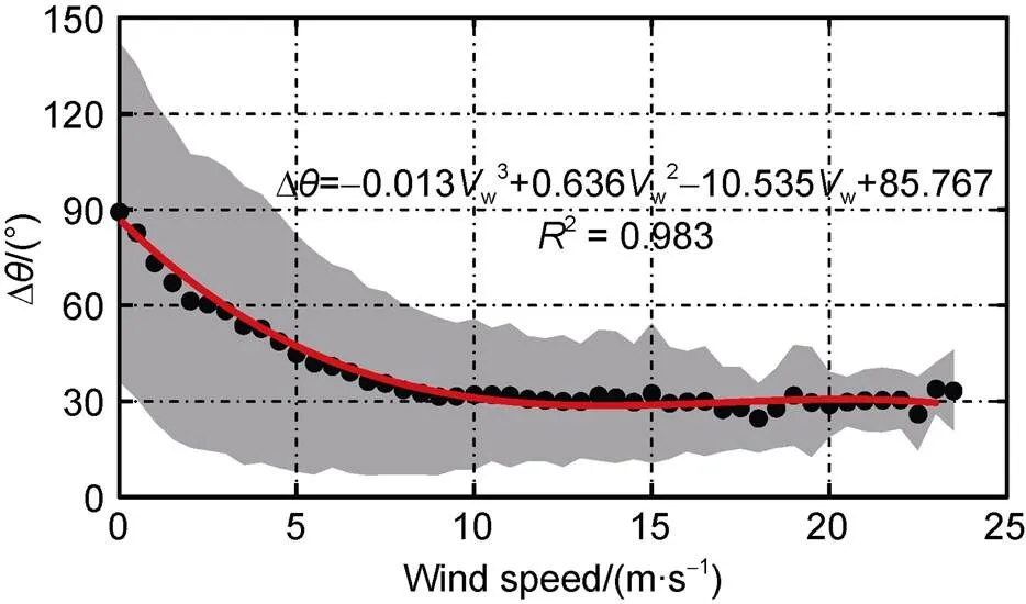
Figure 12 Relationship between mean absolute values of the ice-wind turning angle and 10-m wind speed. The black dots show the mean absolute value of the turning angle between the ice drift and the wind vector, calculated from all buoy data, while the gray shading indicates one standard deviation from the mean, and the red line is the cubic polynomial regression curve.

3.4 Characteristics of ice drift response to skin temperature

Previous study has revealed that the surface temperatures of the Arctic sea ice undergo strong seasonal change, reaching a maximum close to 0 ℃ in summer and a minimum below −45 ℃ in winter (Lindsay et al., 1994). Seasonal variation of sea ice temperature is expressed as changes in mechanical strength and size distribution of the floe ice. These attributes indirectly affect the velocity field of the sea ice. Here, we establish a relationship between sea ice drift velocity and skin temperature. A linear relationship was observed between the ice drift velocity and skin temperature (Figure 13), in which the ice velocity increased by nearly 2% as skin temperature increased by 10 ℃. Figure 14 shows the relationship between the mean absolute values of the ice-wind turning angle and skin temperature. When the skin temperature was lower than −30 ℃, the ice-wind turning angle decreased with increasing skin temperature. Once skin temperature exceeded −30 ℃, the ice-wind turning angle fluctuated between 30° and 60°. Previous research indicates that the atmosphere-ice-ocean momentum exchange can be described as a function of ice concentration, floe size and drift (Steele et al., 1989). In addition to the impact of external environmental conditions (wind speed, current speed) on the sea ice velocity, ice floe geometry (especially ice thickness) influences sea ice velocity. With increasing ice thickness, the ice moves more slowly (Perrie and Hu, 1997), and the influence of wind on sea ice velocity is reduced because of increased internal stresses (Leppäranta, 2011). Likewise, as ice thickness thins under increasing temperature, this can indirectly cause an increase in sea ice velocity.

Figure 13 Relationship between ice velocity and skin temperature. The black dots show the mean ice velocity calculated from all buoy data, while the gray shading indicates one standard deviation from the mean. The red line shows their linear relationship obtained using a least-squares method.

Figure 14 Relationship between mean absolute values of ice-wind turning angle and skin temperature. The black dots show the mean absolute values of the turning angle and skin temperature calculated from all buoy data, while the gray shading indicates one standard deviation from the mean. The red line is the cubic polynomial regression curve.

4 Conclusions

Six buoys were deployed within the Arctic Basin during 2012; three of them drifted out of the Arctic Ocean into the Fram Strait after only 7−11 month. The magnitude of their two-hourly buoy-derived ice velocities ranged from 0.01 to 0.80 m·s−1, contrasting with ice velocities of the three buoys (A, B and E) remaining within the Arctic Basin of generally less than 0.4 m·s−1. These velocity values were substantially greater than average ice velocities reported for the entire Arctic Ocean, likely because of the influence of the TDS. By analyzing the monthly ice velocity probability distribution from September 2012 to December 2013 for three buoys (C, D and F), we documented that ice velocity has a strong seasonal change. The ice velocity probability distribution was more dispersed in September, October and November 2012, because ice velocities were typically greater than 0.2 m·s−1.

The ice velocities also exhibited a strong semi-diurnal signal, reflecting the Coriolis force. Complex Fourier transformation of the amplitudes of the sea ice velocities showed that they had a non-symmetric inertial oscillation, with a peak frequency of about −2 cycle·d−1on the Fourier velocity spectrum. This inertial oscillation is related to ice concentrations and internal stress. The amplitude of the semi-diurnal frequency had a stronger signal closer to the marginal ice zone. This reflects the reduction in internal stress at their margins of ice floes.

To study the relationship between ice drift and wind, two parameters were considered, namely the ratio of ice drift to wind speed and the ice-wind turning angle. The relationship between the observed ice velocity and 10-m wind speed was clearly linear, indicating ongoing change in ice velocities related to changes in wind speed. When the 10-m wind speed was less than 3 m·s−1, there was no clear relationship between ice motion and wind speed. Under wind speeds up to 3 m·s−1, the ratio of ice drift to wind speed remained in the range of 0.01–0.02. There were also seasonal changes in the response of ice velocity to wind speed, yielding a smaller correlation coefficient between ice velocity and wind speed in summer than in winter. We found that ice-wind turning angles were also regulated by wind speed. When the wind speed was less than 12 m·s−1, then the ice-wind turning angle decreased with increasing wind velocity. Once wind speeds exceeded 12 m·s−1, the ice-wind turning angle stabilized to around 30°. This is consistent with ice vectors being east of wind directions in the directional range of 20°–30° in the northern hemisphere.

Sea ice temperature affects ice mechanical strength, indirectly affecting the velocity field of the sea ice. Although current technology is unable to obtain sea ice temperatures directly, we used the skin temperature observed by satellites as a proxy to explore its changes with ice velocity. Our analysis showed that ice velocity generally linearly increased with increasing skin temperature. However, the ice-wind turning angle decreased with increasing skin temperature, when the skin temperature was less than −30 ℃. Once skin temperature exceeded −30 ℃, the ice-wind turning angle typically fluctuated between 30° and 60°.

Our study showed that sea ice velocity was dependent upon seasonal changes in both sea ice temperature and wind speed, as well as ice internal stresses and external oceanic currents like the TDS. This study can be useful to explain the dynamics of Arctic sea ice and precisely track the source and fate of Arctic sea ice.

Acknowledgments This research was supported by the National Natural Science Foundation of China (Grant nos. 41876213 and 41722605) and the National Key R&D Program of China (Grant nos. 2017YFE0111400 and 2016YFC14003).

Comiso J C. 2012. Large decadal decline of the Arctic multiyear ice cover. J Climate, 25(4): 1176-1193, doi:10.1175/JCLI-D-11-00113.1.

Gao Y, Sun J, Li F, et al. 2015. Arctic sea ice and Eurasian climate: A review. Adv Atmos Sci, 32(1): 92-114, doi: 10.1007/s00376-014- 0009-6.

Heil P, Fowler C W, Maslanik J A, et al. 2001. A comparison of East Antarctic sea-ice motion derived using drifting buoys and remote sensing. Ann Glaciol, 33(1): 139-144, doi: 10.3189/1727564017818 18374.

Kanamitsu M, Ebisuzaki W, Woollen J, et al. 2002. NCEP-DOE AMIP-II Reanalysis (R-2). B Am Meteorol Soc, 83(11): 1631-1643, doi: 10.1175/BAMS-83-11-1631.

Kwok R. 2000. Recent changes in Arctic Ocean sea ice motion associated with the North Atlantic Oscillation. Geophys Res Lett, 27(6): 775-778, doi: 10.1029/1999gl002382.

Lee S. 2014. A theory for polar amplification from a general circulation perspective. Asia-Pac J Atmos Sci, 50(1): 31-43, doi: 10.1007/s13143- 014-0024-7.

Lei R, Cheng B, Heil P, et al. 2018. Seasonal and interannual variations of sea ice mass balance from the Central Arctic to the Greenland Sea. J Geophys Res-Oceans, 123(4): 2422-2439, doi: 10.1002/2017JC013548.

Leppäranta M. 2011. The drift of sea ice. Berlin, Heidelberg: Springer Press.

Lindsay R W, Rothrock D A. 1994. Arctic sea ice surface temperature from AVHRR. J Climate, 7(1): 174-183, doi: 10.1175/1520- 0442(1994)007<0174:asistf>2.0.co;2.

Martin T, Augstein E. 2000. Large-scale drift of Arctic sea ice retrieved from passive microwave satellite data. J Geophys Res-Oceans, 105(C4): 8775-8788, doi: 10.1029/1999jc900270.

Maslanik J, Drobot S, Fowler C, et al. 2007. On the Arctic climate paradox and the continuing role of atmospheric circulation in affecting sea ice conditions. Geophys Res Lett, 34(3): L03711, doi: 10.1029/2006GL 028269.

Ogi M, Rigor I G. 2013. Trends in Arctic sea ice and the role of atmospheric circulation. Atmos Sci Lett, 14(2): 97-101, doi:10.1002/ asl2.423.

Olason E, Notz D. 2014. Drivers of variability in Arctic sea-ice drift speed. J Geophys Res-Oceans, 119(9): 5755-5775, doi: 10.1002/2014JC 009897.

Park H S, Stewart A L. 2015. An analytical model for wind-driven Arctic summer sea ice drift. The Cryosphere Discuss, 9(2): 2101-2133, doi: 10.5194/tcd-9-2101-2015.

Perrie W, Hu Y. 1997. Air-ice-ocean momentum exchange. Part II: ice drift. J Phys Oceanogr, 27(9): 1976-1996, doi: 10.1175/1520-0485 (1997)0272.0.CO;2.

Polyakov I V, Timokhov L A, Alexeev V A, et al. 2010. Arctic Ocean warming contributes to reduced polar ice cap. J Phys Oceanogr, 40(12): 2743-2756, doi:10.1175/2010JPO4339.1.

Rampal P, Weiss J, Marsan D. 2009. Positive trend in the mean speed and deformation rate of Arctic sea ice, 1979-2007. J Geophys Res-Oceans, 114(C5): C05013, doi: 10.1029/2008JC005066.

Rigor I G, Wallace J M, Colony R L. 2002. Response of sea ice to the Arctic Oscillation. J Climate, 15(18): 2648-2663, doi: 10.1175/1520- 0442(2002)015<2648:ROSITT>2.0.CO;2.

Schweiger A, Lindsay R, Zhang J, et al. 2011. Uncertainty in modeled Arctic sea ice volume. J Geophys Res-Oceans, 116: C00D06, doi: 10.1029/2011JC007084.

Steele M, Morison J H, Untersteiner N. 1989. The partition of air-ice-ocean momentum exchange as a function of ice concentration, floe size, and draft. J Geophys Res-Oceans, 94(C9): 12739-12750, doi: 10.1029/jc094ic09p12739.

Stoudt C A. 2015. Sea ice near-inertial response to atmospheric storms. University of Alaska Fairbanks, Master Thesis, 12.

Thorndike A S, Colony R. 1982. Sea ice motion in response to geostrophic winds. J Geophys Res-Oceans, 87(C8): 5845, doi: 10.1029/jc087ic 08p05845.

Vihma T. 2014. Effects of Arctic sea ice decline on weather and climate: A review. Surv Geophys, 35(5): 1175-1214, doi: 10.1007/s10712-014- 9284-0.

Vihma T, Launiainen J, Uotila J. 1996. Weddell Sea ice drift: Kinematics and wind forcing. J Geophys Res-Oceans, 101(C8): 18279-18296, doi: 10.1029/96jc01441.

Vihma T, Tisler P, Uotila P. 2012. Atmospheric forcing on the drift of Arctic sea ice in 1989-2009. Geophys Res Lett, 39(2): L02501, doi: 10.1029/2011GL050118.

Weiss J. 2013. Drift, deformation, and fracture of sea ice: A perspective across scales. Berlin, Heidelberg: Springer Press.

Zhang J, Lindsay R, Schweiger A, et al. 2012. Recent changes in the dynamic properties of declining Arctic sea ice: A model study. Geophys Res Lett, 39(20): L20503, doi: 10.1029/2012GL 053545.

Zhang J, Thomas D R, Rothrock D A, et al. 2003. Assimilation of ice motion observations and comparisons with submarine ice thickness data. J Geophys Res-Oceans, 108(C6): 3170, doi: 10.1029/2001JC 001041.

Zhao Y, Liu A K. 2007. Arctic sea-ice motion and its relation to pressure field. J Oceanogr, 63(3): 505-515, doi: 10.1007/s10872-007-0045-2.

24 May 2019;

7 August 2019;

6 March 2020

: Han H W, Lei R B, Lu P, et al. Features of sea ice motion observed with ice buoys from the central Arctic Ocean to Fram Strait. Adv Polar Sci, 2020, 31(1): 26-35,

10.13679/j.advps.2019.0020

, E-mail: leiruibo@pric.org.cn

10.13679/j.advps.2019.0020