Non-random vibration analysis for general viscous damping systems
2020-01-09ChaoJIANGLongLIUJinwuLIBingyuNI
Chao JIANG, Long LIU, Jinwu LI, Bingyu NI
State Key Laboratory of Advanced Design and Manufacturing for Vehicle Body, College of Mechanical and Vehicle Engineering, Hunan University, Changsha 410082, China
Abstract The authors recently developed a kind of non-probabilistic analysis method, named as‘non-random vibration analysis’, to deal with the important random vibration problems, in which the excitation and response are both given in the form of interval process rather than stochastic process.Since it has some attractive advantages such as easy to understand,convenient to use and small dependence on samples, the non-random vibration analysis method is expected to be an effective supplement of the traditional random vibration theory. In this paper, we further extend the nonrandom vibration analysis into the general viscous damping system,and formulate a method to calculate the dynamic response bounds of a viscous damping vibration system under uncertain excitations. Firstly, the unit impulse response matrix of the system is obtained by using a complex mode superposition method. Secondly, an analytic formulation of the system dynamic response middle point and radius under uncertain excitations is derived based on the Duhamel’s integral, and thus the upper and lower response bounds of the system can be obtained.Finally,two numerical examples are investigated to demonstrate the effectiveness of the proposed method.
KEYWORDS Complex mode;Dynamic response bounds;Interval process;Random vibration;Viscous damping system
1. Introduction
In practical engineering problems,the physical parameters and loads of a structure are often uncertain because of the defects of the structure and the disturbances of the external environment. Traditionally, the probability model1,2is used to quantify the uncertainties, where the uncertain parameters are identified by random variables. A great amount of samples are then required to construct precise probability distributions for uncertain parameters. However, it is often challenging to obtain sufficient samples due to either limitations in experiment conditions or cost in practical projects. Therefore, some assumptions have to be made to construct the probability distribution functions of uncertain parameters when using the probability model in practical engineering. Nevertheless,researches have indicated that even a small deviation of the parametric probability distribution may lead to a large error of the structural uncertainty analysis.3
In order to deal with the uncertain problems with limited samples, a variety of non-probabilistic analysis methods4-8have been developed.Among them,the convex model theory5,6treats the uncertain domain of parameters as a convex set that can be easily obtained only based on limited samples or just the engineers’ experience, which thus greatly reduces the dependence on the sample size. In the early 1990s, Ben-Haim and Elishakoff5,6firstly introduced the convex model into uncertainty analysis of structures.After that,the convex model theory has been rapidly developed, and a variety of convex models have been proposed for uncertainty modeling, among which the interval model and the ellipsoid model are the two most widely used ones. Based on the interval model, a series of numerical algorithms were developed to analyze the steady-state response and eigenvalue problems of structures subjected to uncertainty.9,10Based on the second-order truncation model, an error estimation method was proposed for interval and subinterval analysis.11An improved interval analysis method was proposed for structural damage identification.12In addition, a correlation analysis technique was proposed for uncertainty modeling of the multidimensional ellipsoid model.13By using the semi-definite optimization algorithm, the construction of the minimum-volume ellipsoidal convex model under a given set of sample data was studied.14Based on the ellipsoid model, an inhomogeneous eigenvaluebased method was proposed to efficiently predict the bounds of steady dynamic response of dynamic structures under uncertain loads.15By combining interval analysis with the finite element method,the interval finite element method was proposed to compute the structural response bounds under parameters’uncertainties.16,17In recent years, several new convex models,such as the super ellipsoid model,18the multi-ellipsoid model19,20and the multidimensional parallelepiped model,21,22have been proposed successively to deal with more complex uncertain problems.With the growing up of the convex model theory,some related structural uncertainty analysis and design methods were also developed, such as non-probabilistic reliabilityanalysis,23,24uncertainoptimization25,26and probabilistic-convex model hybrid uncertainty analysis,27-29etc.
In existing studies, the convex model theory and corresponding analysis methods are mostly developed for timeinvariant uncertain problems, where the involved parameters and their uncertainties do not change with time. However,the uncertain parameters in practical engineering often have time-varying characteristics such as the wave loads on sailing ships and the road excitations on driving vehicles.To deal with this matter, the interval model was recently extended by the authors into the time-variant problems, and a new mathematical model was proposed to conduct the time-variant or dynamic uncertainty analysis, namely the interval process model.30,31In the interval process model, an interval rather than a precise probability distribution is used to depict the parametric uncertainty at each time point, and hence the uncertainty of the time-varying parameter can be described by two boundary functions over the entire time history. The dependence of the uncertainty quantification on the sample size can thus be reduced to a large extent compared with the traditional stochastic process model.32,33On this basis, a kind of non-probabilistic analysis method for solving the random vibration problems was further developed by the authors through combining the interval process model with the traditional vibration theory,which is named‘non-random vibration analysis’31,34to distinguish from the classical random vibration theory.In non-random vibration analysis, the interval process model is introduced to deal with the uncertain excitation, and hence the response of the vibration system can be also described through an interval process, which is composed of two time-history response bounds. In practical engineering, it seems very easy and intuitive for engineers to use the dynamic response bounds to conduct the reliability analysis and design of a vibration system. Therefore, the non-random vibration analysis method is expected to provide a beneficial supplement to the traditional random vibration theory. So far, some progresses have been made on this method.Two numerical methods were proposed to calculate the dynamic response bounds of the linear Multi-Degree-Of-Freedom (MDOF) vibration systems.31,34A Monte Carlo simulation method was presented to obtain the system’s dynamic response bounds under interval process excitations, providing a general tool for non-random vibration analysis.35An analytical formulation of the dynamic response bounds was derived for non-random vibration analysis based on the Duhamel’s integral.36In the above mentioned works, however, the system damping is assumed to be a proportional damping, with the premise of which the system can be decoupled in the real domain.Based on the real modal theory, the dynamic response bounds of a proportional damping system under uncertain excitations can be deduced, which would have some limitations in practical applications due to the precondition of proportional damping.For the general viscous damping system that exists widely in practice, the system damping is usually no longer a proportional damping, which means that the response bounds of the system generally can’t be accurately obtained by the existing method.Thus,establishing a convincing calculating method of the dynamic response bounds for the general viscous damping system is a significant task regarding the engineering practicability of non-random vibration analysis.
Therefore, this paper extends the non-random vibration analysis method into the general viscous damping system,and formulates a method to calculate the dynamic response bounds for the system under uncertain excitations. The remainder of this paper is arranged as follows:Section 2 introduces the fundamentals of interval process model. Section 3 presents the construction of the non-random vibration analysis method for a general viscous damping system. Section 4 demonstrates the validity of the proposed method by investigating two numerical examples. Finally, Section 5 gives the conclusions.

Fig.1 The interval process.31
2. Fundamentals of interval process model30,31
As shown in Fig. 1, the interval process model30,31employs a bounded and closed interval for quantification of the parametric uncertainty at arbitrary time point,and an auto-covariance function is defined to describe the correlation between the interval variables at arbitrary two different time points.
Definition 1. A time-varying uncertain parameter{X (t ), t ∈T} is an interval process if for arbitrary time ti∈T, i=1,2,..., the possible values of X(ti) can be represented by an interval XI(ti)=[XL(ti),XU(ti)], where T is a parameter set of t.
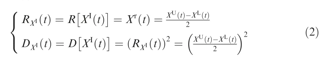
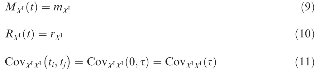
Definition 2. For an interval process XI(t ) with the upper bound function XU(t ) and the lower bound function XL(t ),the middle point function of XI(t ) is defined as:

Definition 3. For an interval process XI(t ) with the upper bound function XU(t )and the lower bound function XL(t ),the radius function RXI( t) and the variance function DXI( t) of XI(t ) are defined as:
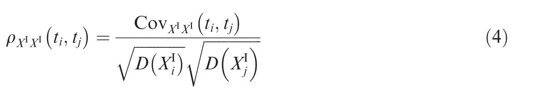
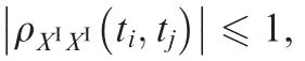
Definition 4. For an interval process XI(t ),the auto-covariance function of interval variables XI(ti)and XItjat any two time points tiand tjis defined as:

where θ is the relevant angle, r1and r2are the half lengths of the major axis and the minor axis of the ellipse, and they can be obtained based on the samples of XI(t ), as shown in Fig. 2, and more details on the construction of an ellipsoid uncertain domain can refer to our previous works.13,30For ease of expression, in this paper we also denote X(ti) as Xi,XI(ti) asandin brief. From the definition of auto-covariance function, it is not difficult to prove thatand

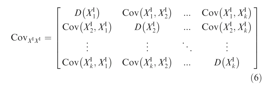
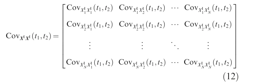
As shown in Fig.2,in the interval process model the correlation of the interval variables at any two time points is described through an ellipse, and this ellipse also represents the uncertainty domain of these two interval variables in the two-dimensional variable space. Thus, a multidimensional ellipsoid can be introduced to describe the uncertainty domain of the interval variables at multiple time points. Namely, for variables X1∈X2∈...,Xk∈at any k time points of XI(t ), its k-dimensional uncertainty domain Ω can be expressed by a hyper-ellipsoid:
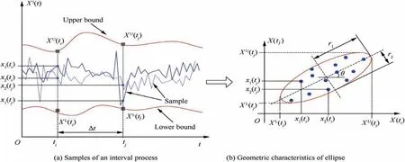
Fig.2 Calculation of auto-covariance function of interval process.36

where Xmdenotes a k-dimensional interval middle point vector, and CovXIXIdenotes the auto-covariance matrix of XI(t )defined as:
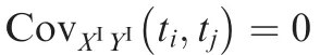
Definition 6. The cross-covariance function of two interval processesandis defined as:

Definition 7. The cross-correlation coefficient function of two interval processes XI(t ) and YI(t ) is define as:
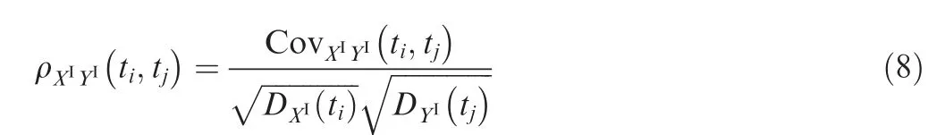


Fig.3 Calculation of the cross-covariance function of two interval processes.36
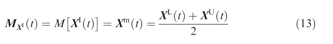
Definition 10. For an interval process vector XI(t ) with the upper bound function vector XU(t ) and the lower bound function vector XL(t ), the middle point function vector of XI(t ) is defined as:
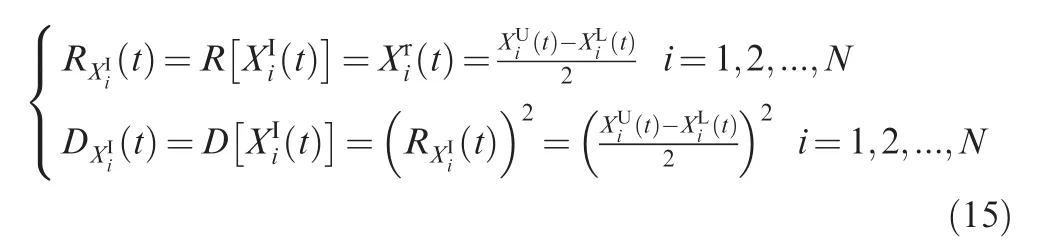
Definition 11. For an interval process vector XI(t ) with the upper bound function vector XU(t ) and the lower bound function vector XL(t ), the radius function vector RXI(t )and the variance function vector DXI(t ) of XI(t ) are defined as:
where
3.Dynamic response bounds of general viscous damping systems
By introducing the interval process model30,31to describe the uncertain excitation, the authors recently developed a kind of non-probabilistic analysis method, named as ‘non-random vibration analysis’,31,34to deal with the random vibration problems. In order to enhance the applicability of nonrandom vibration analysis, this paper further extends the non-random vibration analysis method into the general viscous damping system, and deduces the dynamic response bounds for the system under dynamic uncertain excitations.In this section, the state space method37is firstly introduced to decouple the general viscous damping system in the complex domain. Then, the dynamic response bounds for the system under uncertain excitations are derived based on the complex mode superposition theory.
3.1. The state space method
In case of the general viscous damping system that exists widely in structural vibration problems, the damping matrix generally does not satisfy the orthogonal condition of the real modal theory. In this case, the system generally cannot be decoupled in the real domain, and the dynamic response for the general viscous damping system usually cannot be accurately obtained based on the real modal theory. As a generalization of the real modal theory,the complex modal theory can realize the decoupling of arbitrary viscous damping systems in the complex modal space.38In this section, the state-space method is applied to decouple the general viscous damping system in the complex domain, and the complex modal parameters of the system can then be obtained.
The free vibration equations of a general viscous damping system are expressed as:39
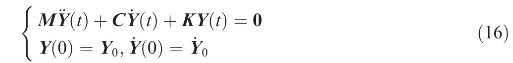
where M,C and K are n×n mass matrix,damping matrix and stiffness matrix, respectively; Y(t), ˙Y(t)and ¨Y(t) are ndimensional displacement, velocity and acceleration vectors,respectively; Y0and ˙Y0represent the displacement vector and the velocity vector at the initial moment, respectively.The eigenvalue equation for Eq. (16) is:

where λ and φ are the eigenvalue and the eigenvector, respectively. Since Eq. (16) cannot be decoupled in physical coordinates, another kind of coordinate description, namely the state space description is considered.The 2n-dimensional state vector composed of displacement vector and velocity vector is introduced:

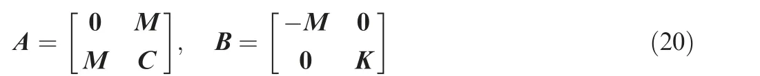
Eq.(16)can then be written as a set of first-order linear differential equations described by the state vector:

where
The eigenvalue equation for Eq. (19) is:

where λ and Ψ are the eigenvalue and the eigenvector, respectively.According to the literature40,the eigenvalues of Eq.(17)and Eq. (21) are the same, namely λi(i=1,2,···,2n) and the eigenvectors have the following relationship:

And the 2n-dimensional complex eigenvectors, namely Ψi(i=1,2,···,2n) are linearly independent of each other,indicating that they can be used as the basis vectors. Then,the following transformation function is introduced:
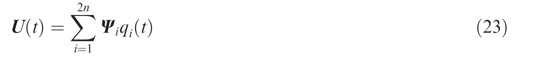
Substituting Eq.(23)into Eq.(19)and premultiplying both sides of Eq. (19) by ΨTi , 2n decoupled first-order differential equations can be obtained:

where
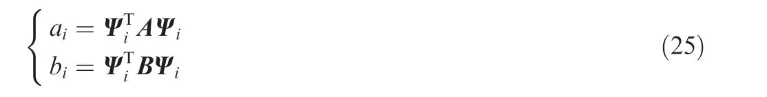
Substituting Eq.(23)into Eq.(16)and premultiplying both sides of Eq. (16) by ΨTi A, the solution of Eq. (24) can be obtained:
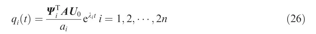
where
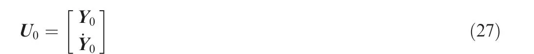
Substituting Eq. (26) into Eq. (23), the free vibration responses described by the physical coordinate can be obtained:
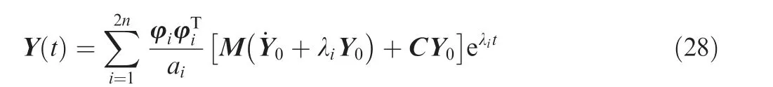
The motion equation for the general viscous damping system subjected to external excitations is given by39:

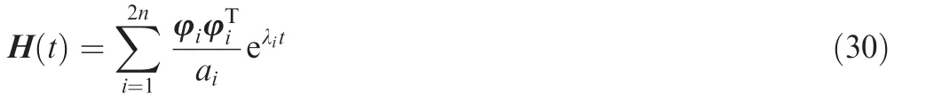
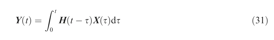
where X(t ) is the n-dimensional external excitation vector.According to Eq. (28), supposing the initial condition of ˙Y(0)=0, Y(0)=0, the unit pulse response matrix of the system can be obtained:
the dynamic responses for the general damping system under external excitations can then be obtained based on the Duhamel’s integral41as:
3.2. Calculation of dynamic response bounds
When the excitations applied to the system are uncertain and described as an interval process vector XI(t), the dynamic responses of the system can be also described as an interval process vector:

According to the interval process theory,31the response bound function can be determined by the middle point function and the radius function. Therefore, the upper and lower bounds of the dynamic responses can be obtained by solving the middle point function and the radius function of the system responses.kno wn that M[·] is a linear operator from the literature.36By
Denote M[·] as the middle point operator, and it can be performing the middle point operation on the response function YI(t) in Eq. (32), the middle point function vector of YI(t) can be obtained:
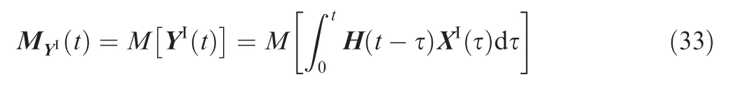
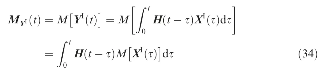
Since M[·]is a linear operator whose operation order can be changed with the integral operator, the middle point function vector is:
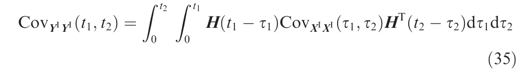
According to Eq. (2), the radius function is obtained by taking the root of the variance function,namely the covariance with itself at a certain moment of the interval process. Therefore, the radius function of the system response can be indirectly obtained through its covariance function. According to the literature,36the cross-covariance function matrix of YI(t),namely CovYIYI(t1,t2) can be expressed as:
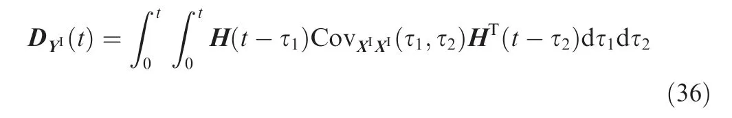
Then, the radius function vector of YI(t ) can be obtained:
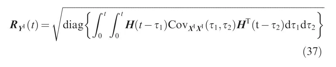
where diag{·}denotes taking the diagonal terms of the matrix.According to MYI(t )and RYI(t ),the dynamic response bounds can then be obtained:
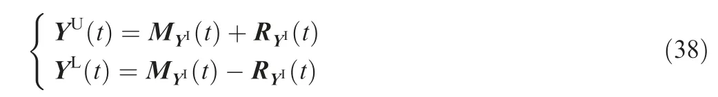
where YU(t) and YL(t) represent the upper and lower bounds of the dynamic responses for the general viscous damping system, respectively.
4. Numerical examples and discussions
For a general viscous damping system, the modal damping matrix is no longer a diagonal matrix,and the system response cannot be accurately calculated by the traditional real modal analysis method. By neglecting the off-diagonal elements of the modal damping matrix, the forcing decoupling method37can be applied to realize the approximate decoupling of the system, and then an approximate solution of the dynamic response for the system can be acquired by the Duhamel’s integral. Based on the forcing decoupling method, the existing method can be applied to calculate the dynamic response bounds of the general viscous damping system under uncertain excitations, which certainly would deviate from the actual results to a certain extent due to the ignoring to the nondiagonal elements. In this paper, however, the general viscous damping system is decoupled in the complex domain by using a complex mode superposition method, and an analytic solution of dynamic response bounds for the general viscous damping system under uncertain excitations is deduced.In this section, the proposed method and the existing method are respectively used to compute the dynamic response bounds of two numerical examples, and the validity of the proposed method is verified.
4.1. A 2-DOF vibration system
Consider a 2-DOF viscous damping vibration system subjected to two external excitations x1(t) and x2(t),as shown in Fig.4,whose mass matrix, damping matrix and stiffness matrix are respectively expressed as:
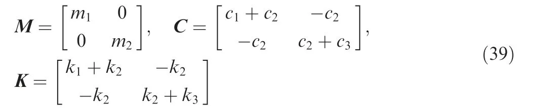
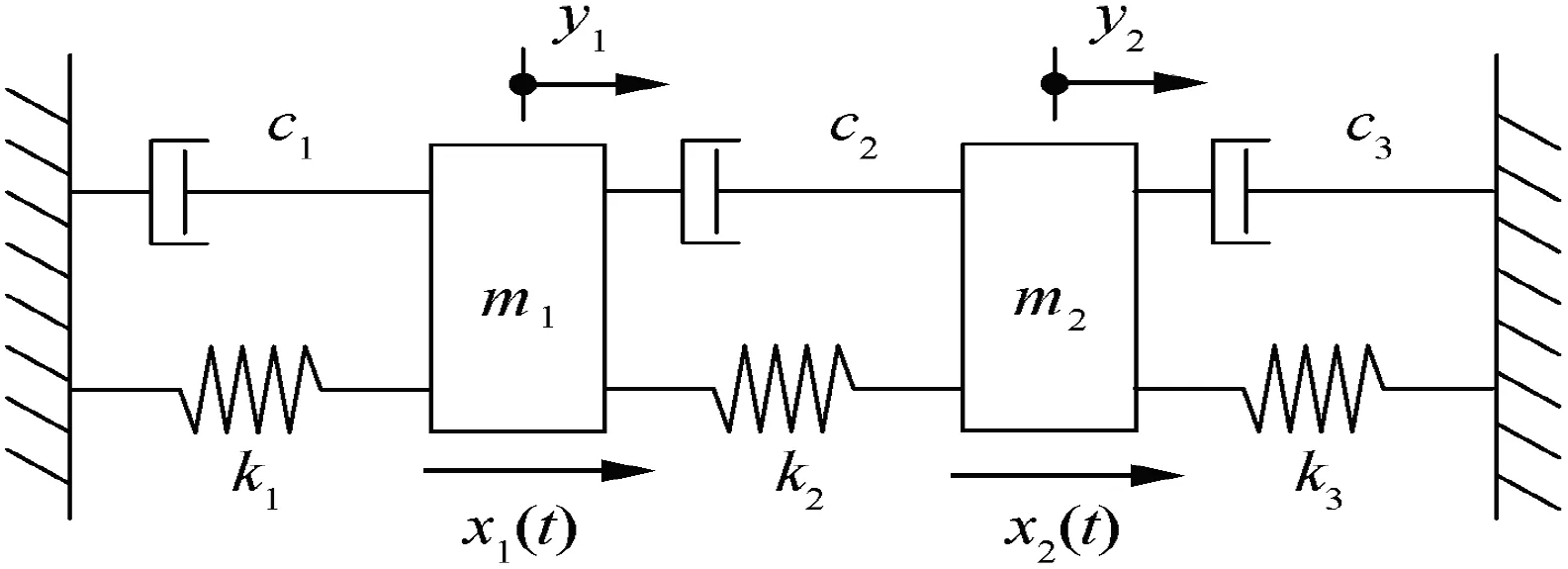
Fig.4 The 2-DOF vibration system.39
where m1=1, m2=2, k1=k2=k3=10, c1=1.5, c2=0.5,c3=0.5. Both the two external excitations are treated as stationary interval processes, where the middle point and radius functions are respectively(t )=2.5,(t )=5,(t )=2 and(t )=4, the auto-correlation coefficient functions are ρ1(τ )=e-|τ|cos(2 τ) and ρ2(τ )=e-2|τ|cos(2 τ), respectively. In addition, four kinds of cross-correlation coefficient functions are considered for the two interval process excitations,namely,and
Firstly, effects of different types of cross-correlation coefficient functions between the two excitations on the system response bounds are studied. By applying the proposed method to calculate the dynamic response bounds of the system under the two excitations, the time history curves of the response bounds under four cases of cross-correlation coefficient functions are obtained, as shown in Fig. 5. According to Fig.5,the dynamic response bounds of y1(t )and y2(t )under the four different cross-correlation coefficient functions can be roughly divided into two stages,namely the transient response stage and the steady-state response stage. In the transient response stage, the middle point and radius functions both fluctuate with time, and the response bounds present obvious oscillation that tends to be slighter with time,reaching a steady state eventually. In the steady-state stage, both the middle point and radius of the response keep almost constant.Besides, different cross-correlations between excitations have some influence on the system response bounds under given excitations. For the four different cross-correlation coefficient functions, the response intervals of y1(t ) and y2(t ) in the steady-state stage are given in Table 1.It can be observed that under the four different cross-correlation coefficient functions,the steady-state response middle points of y1(t ) are all 0.3333 and the radii are 0.4464, 0.4913, 0.5434 and 0.3650, respectively. Correspondingly, the steady-state response middle points of y2(t ) are all 0.4167 and the radii are 0.5739, 0.6389,0.6661 and 0.5015, respectively. Thus, the four different cross-correlation coefficient functions would only have influence on the response radii without affecting the middle points for the system under given excitations. Moreover, for the four given cross-correlation coefficient functions between x1(t) and x2(t), the steady-state response radius of y1(t ) and y2(t ) are both the smallest when the cross-correlation coefficient function is zero, which means that the resulting steady-state response intervals are the narrowest.

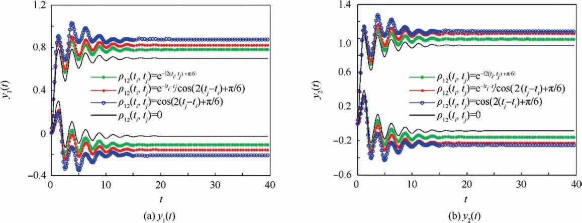
Fig.5 Displacement response bounds of the 2-DOF system under different cross-correlation coefficient functions.
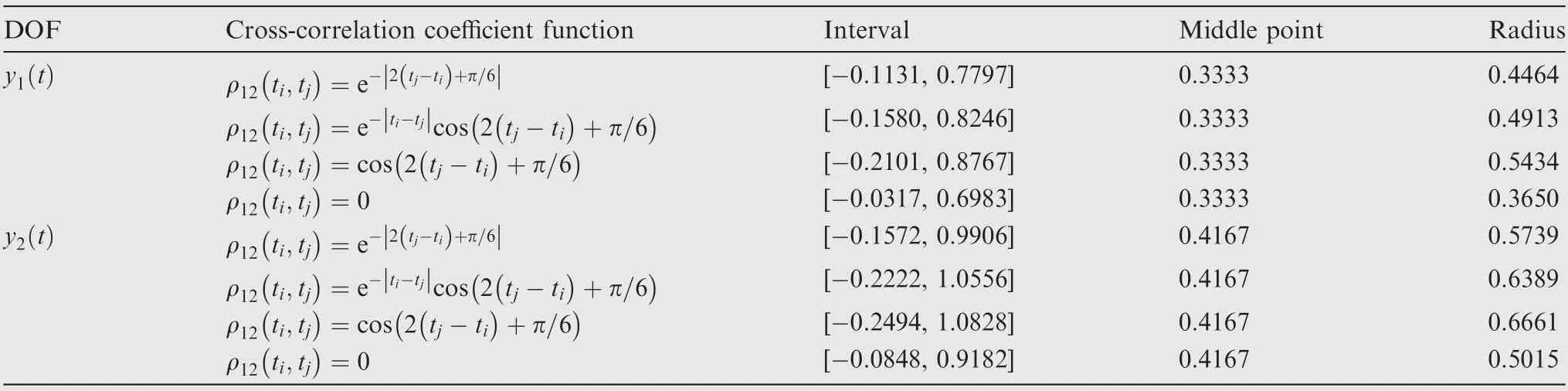
Table 1 Displacement response bounds of 2-DOF system in steady-state response stage under different cross-correlation coefficient functions.
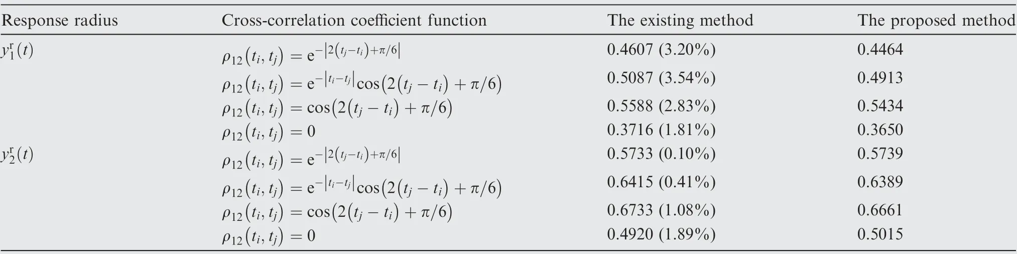
Table 2 The comparison between response radii of the 2-DOF system in steady-state response stage under different cross-correlation coefficient functions.
4.2. An 8-DOF vehicle vibration problem
Driving vehicles are usually influenced by the time-varying uncertain vibration induced by the road excitation, which would affect traffic safety, ride comfort and handling stability.42Therefore, it is necessary to analyze the dynamic responses of vehicles under time-varying uncertain excitations.In order to analyze the influence of the dynamic uncertain excitation on the vibration response of the vehicle system, an 8-DOF vehicle vibration system43is considered, as shown in Fig. 6. The parameters of the vehicle system are summarized in Table 3.Assuming that the car is moving at a constant speed of v=20 m/s, the dynamic equation of the vibration system can be expressed as:

where M,C,K are 8×8 matrixes,whose specific forms can refer to43. The tire stiffness matrix is given by:
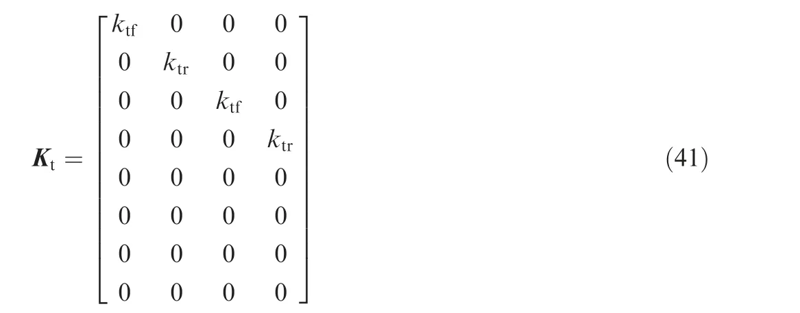
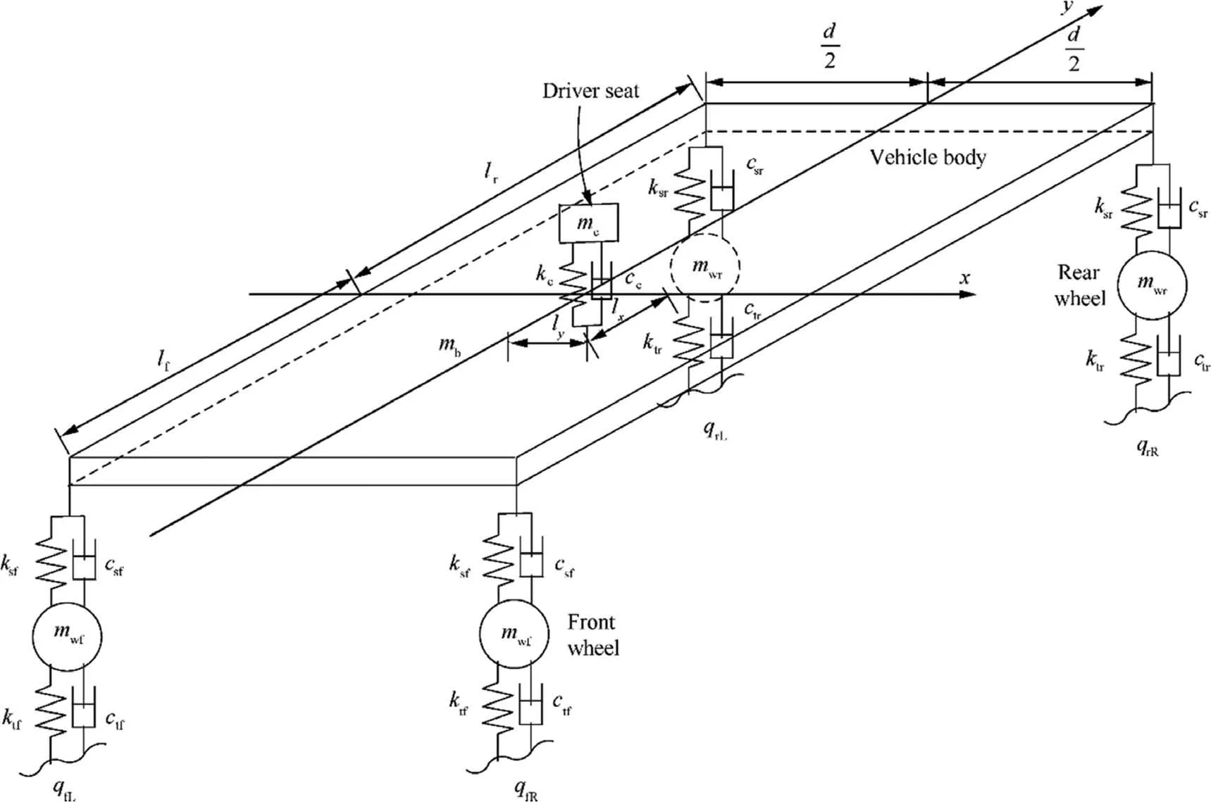
Fig.6 The 8-DOF vehicle vibration model.43
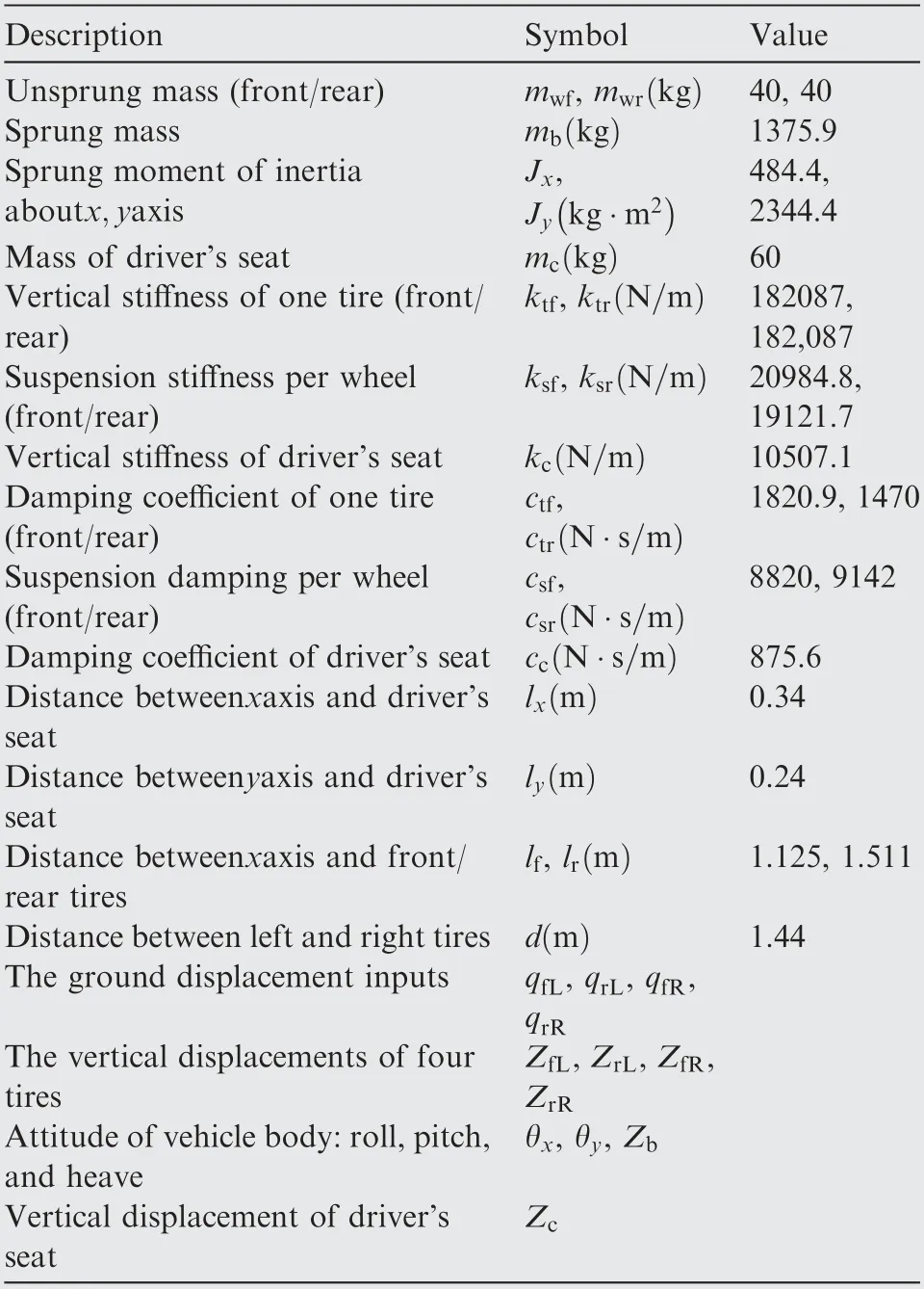
Table 3 The involved parameters of 8-DOF vehicle vibration system.
The excitation vector Q caused by the road is:

The response vector Y is:

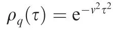
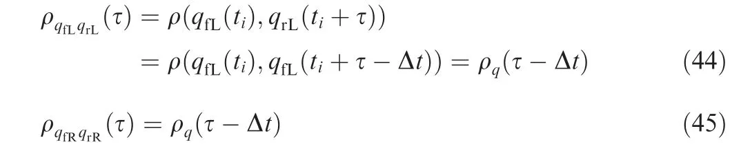
It is assumed that the uncertain excitations on the left and right tires are independent, which means that the crosscorrelation coefficient functions of the excitations on left and right tires are set as 0, namely:

By using the proposed method, the dynamic response bounds of the vehicle vibration system are obtained,as shown in Fig.7.According to Fig.7,each response gradually reaches a steady state after experiencing an initial non-stationary phase. Among the 8 DOFs, the four vertical displacement responses of tires, namely ZfL(t ), ZrL(t ), ZfR(t ) and ZrR(t ),reach stable faster than the other four DOFs that gradually entered the steady state within 0.4 s. Since the middle points of the excitations are zero at any time,the middle point of each response of the system is also always zero.The intervals of the 8 DOFs in the steady-state response stage are given in Table 4.It can be found that the intervals of the vertical displacement responses of the four tires are very close, which indicates that the overall level of vehicle turbulence is roughly the same when the vehicle runs at a speed of 20 m/s on the road.Besides, the response intervals of the front tires are slightly wider compared with those of the rear rears, indicating that the vibration amplitudes that the front wheels can reach would be a little larger. The steady-state intervals of the vertical displacement of the vehicle body and the vertical displacement of the driver’s seatarerespectively[-2.48 cm,2.48 cm]and [-3.19 cm,3.19 cm], which means that the maximum amplitudes that the two responses may reach during the driving process are 2.48 cmand 3.19 cm, respectively. By comparing the vertical displacement of the vehicle body with the vertical displacements of the four wheels, it is found that the vertical displacement of the vehicle body is obviously smaller, which shows that the suspension system of the vehicle has a prominent effect on vibration reduction. In addition, the attainable maximum amplitudes for the pitch and roll angles of the vehicle body are 1.88° and 0.97° respectively, indicating that the vehicle would rarely roll or pitch at 20 m/s on the road.
Moreover,the existing method is used to solve the dynamic response bounds of the 8-DOF vehicle vibration system, and the steady-state results obtained are compared with those of the proposed method,as shown in Table 5.It can be seen that the steady-state response radii of the four tires obtained by the existing method are 3.52 cm, 3.50 cm, 3.51 cm and 3.50 cm respectively, whose relative errors are 28.28%, 25.86%,28.64% and 25.60%, respectively. For the other responses,namely Zb, θx, θyand Zc, the steady-state response radii obtained by the existing method are 1.13 cm, 0.87°, 0.15°and 1.19 cm respectively, and the relative errors all exceed 50%, where that of θyis the largest, reaching 84.64%.
Based on the two result comparisons, it can be found that the steady-state response bounds obtained by the existing method for the 2-DOF vibration system have a slight deviation,while for the 8-DOF vehicle vibration system,the relative error of each response is quite large. Therefore, the existing method cannot accurately calculate the dynamic response bounds of the system when dealing with a general viscous damping system.Especially for complex engineering problems,where the system has more degrees of freedom and the nondiagonal elements of the modal damping matrix greatly affect the result,the accuracy of the existing method will not be able to satisfy the engineering demand. Nevertheless, the proposed method is a rigorous calculating method based on the complex modal superposition theory,and the dynamic response bounds of a general viscous damping system can be obtained, which are more convincing for the analysis of practical engineering problems.
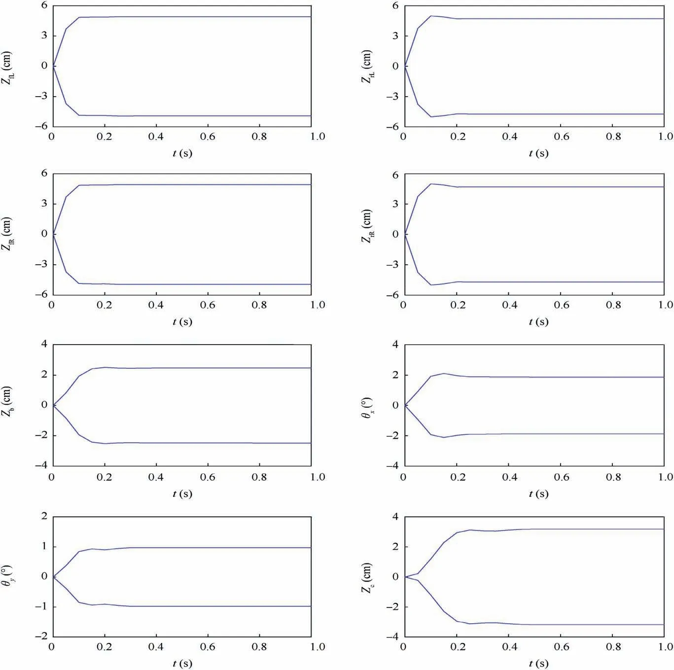
Fig.7 Dynamic response bounds of the 8-DOF vehicle vibration system.

Table 4 Response bounds of 8-DOF vehicle vibration system in steady-state response stage.
5. Conclusions
In this paper,a non-random vibration analysis method for the general viscous damping system is proposed, and the dynamic response bounds of the system under dynamic uncertain excitations can be obtained. In this method, the interval process rather than the stochastic process is used to describe the dynamic uncertain excitation,which greatly reduces the dependence of the uncertainty quantification on the sample size.Based on the complex modal superposition theory, the decou-pling of the general viscous damping system is implemented in the complex domain, and the dynamic response bounds of the system under uncertain excitations can be obtained.According to the results of two numerical examples,the dynamic response bounds of the system obtained by the existing method would deviate from the actual bounds when dealing with a general viscous damping system under dynamic uncertain excitations.Moreover, the deviation may be considerably large with the increase of system freedom degrees. However, the proposed method that is based on the complex modal superposition theory can well solve the dynamic response bounds of the general viscous damping system subjected to dynamic uncertain excitations identified by interval processes. Besides, the dynamic response bounds can provide an important reference for the safety evaluation and reliability design of practical vibration systems.
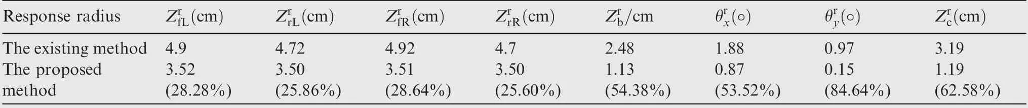
Table 5 The comparison between response radii of 8-DOF vehicle vibration system in steady-state response stage.
Acknowledgements
This work is supported by the Science Challenge Project of China (No. TZ2018007), the National Science Fund for Distinguished Young Scholars (No. 51725502), the National Key R&D Program of China (No. 2016YFD0701105), the Open Project Program of Key Laboratory for Precision &Non-traditional Machining of Ministry of Education, Dalian University of Technology of China (No. JMTZ201701).
杂志排行

CHINESE JOURNAL OF AERONAUTICS的其它文章
- A CFD-based numerical virtual flight simulator and its application in control law design of a maneuverable missile model
- Numerical investigation of flow mechanisms of tandem impeller inside a centrifugal compressor
- Experimental investigation on dynamic response of flat blades with underplatform dampers
- Numerical analysis of hypersonic thermochemical non-equilibrium environment for an entry configuration in ionized flow
- Prediction of nonlinear pilot-induced oscillation using an intelligent human pilot model
- Multiple hierarchy risk assessment with hybrid model for safety enhancing of unmanned subscale BWB demonstrator flight test