Novel Ensemble Modeling Method for Enhancing Subset Diversity Using Clustering Indicator Vector Based on Stacked Autoencoder

Yanzhen Wang and Xuefeng Yan,

Abstract: A single model cannot satisfy the high-precision prediction requirements given the high nonlinearity between variables.By contrast,ensemble models can effectively solve this problem.Three key factors for improving the accuracy of ensemble models are namely the high accuracy of a submodel,the diversity between subsample sets and the optimal ensemble method.This study presents an improved ensemble modeling method to improve the prediction precision and generalization capability of the model.Our proposed method first uses a bagging algorithm to generate multiple subsample sets.Second,an indicator vector is defined to describe these subsample sets.Third,subsample sets are selected on the basis of the results of agglomerative nesting clustering on indicator vectors to maximize the diversity between subsets.Subsequently,these subsample sets are placed in a stacked autoencoder for training.Finally,XGBoost algorithm,rather than the traditional simple average ensemble method,is imported to ensemble the model during modeling.Three machine learning public datasets and atmospheric column dry point dataset from a practical industrial process show that our proposed method demonstrates high precision and improved prediction ability.

Keywords: Ensemble model,deep learning,bagging,stacked autoencoder,XGBoost.

1 Introduction

Regression,which is frequently used to build mathematical models of complex objects and predict specific output results,has attracted considerable attention in machine learning during the past decades [Vanli,Sayin,Mohaghegh et al.(2019)].In many studies,linear and nonlinear regression and their improved modeling methods based on multivariate statistics and traditional machine learning have been proposed;the modeling methods include ridge regression [Li,Hu,Zhou et al.(2018)],least absolute shrinkage and selection operator regression [Xu,Fang,Shen et al.(2018);Osborne and Turlach (2011)],partial least squares regression [Lavoie,Muteki and Gosselin (2019);Biancolillo,Naes,Bro et al.(2017)],support vector regression (SVR)[Zhang,Gao,Tian et al.(2016);Wei,Yu and Long (2014)],and artificial neural network (ANN)[Du and Xu (2017);Martinez-Rego,Fontenla-Romero and Alonso-Betanzos (2012)].These regression methods have been applied to building mathematical models for various real-life scenarios,such as time series [Safari,Chung and Price (2018);Sarnaglia,Monroy and da Vitoria (2018);Sahoo,Jha,Singh et al.(2019)] and industry [Xue and Yan (2017);Rato and Reis (2018);Sedghi,Sadeghian and Huang (2017);Khazaee and Ghalehnovi (2018);Gonzaga,Meleiro,Kiang et al.(2009)].However,many problems,such as multiple operating conditions and high nonlinearities,interfere with the prediction quality of key variables given the complexity of object processes and high-precision requirement of models.Ensemble models are imported to overcome the overfitting and low generalization ability of a single model [Bidar,Shahraki,Sadeghi et al.(2018)].The significance of an ensemble depends on the formation of a series of submodels.A multilearner system is established through a certain fusion strategy to accomplish the same task as a single model [Kittler,Hatef,Duin et al.(1998)].

At present,various ensemble modeling methods have been developed [Magalhaes (2012);Rajalakshimi,Rengaraj,Bharadwaj et al.(2018);Li,Ge and Zang (2018)].Mohan and Saranya [Mohan and Saranya (2019)] developed a novel bagging ensemble approach using four base learners,namely,multilayer perceptron,RTree,REPTree,and random forest (RF).The forecasting effect on surface-level O3 concentration was accurate by evaluating the errors measured by each submodel.Moretti et al.[Moretti,Pizzuti,Panzieri et al.(2015)] investigated a bagging ensemble model through statistical method and neural network.Whether the submodel output was substituted by ANN or statistical method was determined by the prediction error of submodels.Three cases showed that their model outperforms other parallel methods.Hu et al.[Hu,Mao,He et al.(2011)] presented a novel SVR ensemble algorithm based on bagging and negative correlation learning to compensate for errors.Their model continuously reconstructed the samples of the next submodels to improve the set error.The average value of the predicted output of each submodel was used as the final prediction result.Leaching simulation showed that their model outperforms the three other models.

These studies have achieved favorable results in various applications.However,they have not considered the fundamentals of ensemble models.High accuracy and a significant diversity of submodels are the two key factors for increasing the efficiency of ensemble modeling algorithm [Sun,Wang,Chen et al.(2014)].An ensemble method immensely affects the performance of the entire model.The improvement of the three factors significantly enhances the fitting prediction ability and robustness of the integrated model.For the first factor,most studies have typically adopted traditional multivariate statistical analysis and machine learning algorithms,such as ANN and SVR,as the submodels in the hybrid modeling method.Furthermore,the prediction accuracy of traditional machine learning methods is limited,and the lack of generalization ability leads to poor prediction effect of submodels.As a key research area in artificial intelligence,deep learning,which was first proposed by Hinton and Salakhutdinov [Hinton and Salakhutdinov (2006)],has gradually replaced machine learning algorithms.Deep learning algorithms have a strong nonlinear fitting ability and can effectively overcome gradient diffusion and local optimum caused by ANN.Stacked autoencoders (SAE)are common algorithms used in deep learning [Yuan,Huang,Wang et al.(2018);Yan and Yan (2019)].For the second factor,the bagging algorithm has been extensively adopted to generate multiple subsample sets.Although training subsets with certain differences can be obtained through the bagging algorithm,the diversity and difference between each submodel are determined on the basis of the randomness and independence of resampling a trained subsample set from the bagging algorithm [Sun and Sun (2016)].Accordingly,the distribution of some subsample sets resampled through multiple rounds of bootstrapping might be similar,and their diversity was insignificant.No clear measurement of diversity and difference between subsets has been defined.In addition,the output of each individual submodel is typically produced through a simple or weighted average to produce an ensemble final output when an integrated concept is applied to a regression estimation problem.The two traditional methods ignore the possibility of using a nonlinear function to describe the mathematical relationship between submodels for achieving an improved prediction effect.

Based on these truths,we propose a novel ensemble modeling method to enhance the diversity between subsets using a clustering indicator vector based on bagging and SAE.The agglomerative nesting (AGNES)clustering algorithm is used to cluster the indicator vector of each subsample set after bagging.The number of clusters determines the number of submodels.One subset of each cluster is selected and placed into an SAE for training to obtain the subsets with the most significant diversity.XGBoost algorithm is imported to integrate all the submodels during the model integration phase.

The rest of this paper is organized as follows.Section 2 introduces the basic knowledge and algorithms.Section 3 describes our proposed modeling method in detail.Section 4 presents the results and analysis of parallel comparative experiments on three public datasets and one dataset from a practical industrial process.Section 5 provides the conclusion drawn from this study.

2 Preliminaries

The basic knowledge and concepts of bagging algorithm,AGNES,SAE,and XGBoost are briefly reviewed,and an indicator vector is defined to illustrate the diversity of subsample sets in this section.

2.1 Bagging

Bagging,as a common and effective multilearner method,utilizes bootstrap sampling in constructing component learners and generates sufficient independent variance among them [Hu,Mao,He et al.(2011)].Suppose the existence of a labeled datasetD={X,y},whereX∈Rn×m,y∈Rn×1,nis the number of samples,andmexpresses the number of variables.The core idea of the bagging algorithm based on bootstrap resampling is to construct the same size of each subset as the original training sample set by randomly extracting samples from original training samples [Li and Yan (2018)].During resampling,some samples of the original sample dataset may appear several times in the subset,whereas other samples may not emerge.Tsample subsets are achieved by repeatingTrounds of bootstrap resampling,which can be expressed as:Dbagging={D1,D2,...,DT},whereDt= {X t,yt},t∈[1,T],Xt∈Rn×m,andyt∈Rn×1.

2.2 AGNES

AGNES is considered a bottom-up approach to hierarchical clustering.First,each sample is treated as an initial cluster.Second,in each step of the algorithm,two clusters that fit the similarity measurement are aggregated until all objects are merged into a single cluster.Finally,a threshold is determined to select the result of clustering.The detailed steps and selective similarity measurement of the AGNES algorithm can be found in Xie et al.[Xie and Wang (2018);Zhou (2016)].In the present study,the average value of Euclidean distance between two clusters is used as the similarity measurement.In particular,two clusters with the smallest average Euclidean distance value between all samples are merged.

2.3 AE and SAE

AE,which is inspired by ANN,is a typical unsupervised machine learning method.SAEs have been used as the representative algorithms in deep learning since the introduction of a layer-wise greedy training algorithm into AE by Hinton et al.[Hinton and Salakhutdinov (2006)] in 2006.The training mechanism of SAEs is divided into two steps,namely,unsupervised pretraining and supervised fine-tuning.

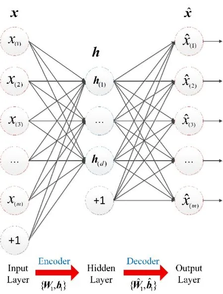
Figure 1:Schematic of the AE

During unsupervised pretraining,each AE in SAEs aims to reconstruct input signals through gradient descent algorithm.Fig.1 illustrated the schematic of the AE.The unlabeled dataset isX= {x1,x2,…,xn},wherexi∈Rm,mdenotes the number of variables,andnis the number of samples.The encoding part,which is formed from the input layer to the hidden layer,extracts the abstract feature of input data.The extracted feature can be denoted asH= {h1,h2,…,hn} ,wherehi∈Rd,andddenotes the number of nodes in the hidden layer.The encoding part can be calculated as

whereW1andb1indicate the weight matrix and bias vector of the encoding portion,respectively.s1(⋅)is the activation function of the network.In this study,all activation functions of our model use a sigmoid function as the activation function,which can be described as follows:

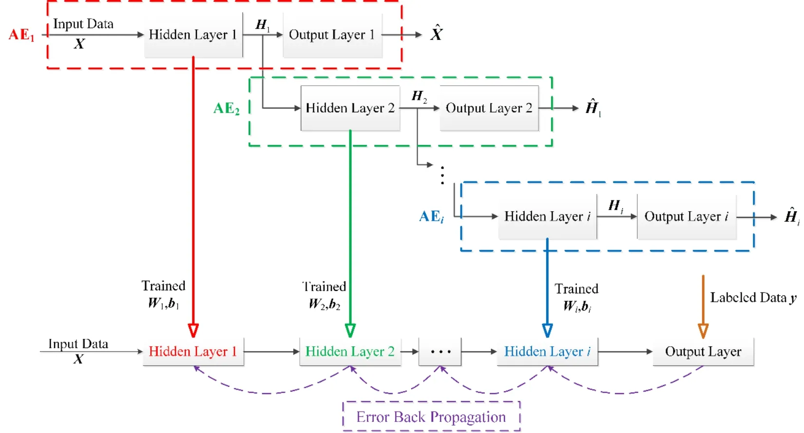
Figure 2:Structure of the SAE

The decoding part is formed from the hidden layer to the output layer to reconstruct the input data.The reconstructed signal can be defined as,where.The decoding part is determined as follows:

Within the allowable range of error,the reconstructed signal in the AE is typically useless and can be ignored.The output of the hidden layer with reduced dimensions becomes an important abstract feature of the original signal.The output of the hidden layer of the previous AE is adopted as the input signal of the next AE,which constitutes the structure of the SAE and can be denoted as

wherefθi(⋅)is the mapping function,andnsis the number of AEs in the SAE.

During supervised fine-tuning,the trained weight matrix and bias vector of each AE denoted as {Wi,bi} are placed in a multilayer deep neural network as the initial values.The nodes of each layer in this network are the same as the number of hidden nodes in each AE.The output of this network is set as the labeled data denoted asy= {y1,y2,…,yn} .Subsequently,a backpropagation algorithm is used to fine-tune the parameters of the entire network and to make the output of this model and labeled data equal.Fig.2 presents the entire structure of the SAE.

2.4 XGBoost

XGBoost,an extension of gradient boosting decision tree (GDBT),is an ensemble learning algorithm proposed by Chen et al.in 2016 [Zhang,Chen,Xu et al.(2019)].In recent years,XGBoost has demonstrated significant regression and classification performance in the Kaggle data-mining competition [Qi,Xu and Zhu (2019)].In comparison with GBDT,which only uses the first-order derivative information during optimization,XGBoost introduces the Taylor second-order derivative and expands the target loss function to improve calculation accuracy.In addition to the loss function,XGBoost finds the optimal solution for the regular term.Simultaneously,XGBoost has a built-in cross-validation feature sampling and regularization that can extremely prevent overfitting.Mean square error (MSE)is imported as the target function when solving regression problems.XGBoost can automatically use a CPU’s multithreaded calculations,thereby reducing runtime and improving algorithm accuracy.Zhou et al.[Zhou,Li,Shi et al.2019] provided a detailed derivation and calculation method of the XGBoost algorithm.

2.5 Indicator vector

We define a simple and intuitive variable called an indicator vector to describe the matrix distribution intuitively.Statistically,the mean and variance values are frequently used to exhibit the distribution of vectors.Thus,we extend the two symbols to define the diversity between matrixes.The existence of an unlabeled datasetX={x1,x2,…,xn} ，xi∈Rmis assumed.The formula of mean and variance for thejth independent variable can be expressed using Eqs.(6)and (7).

The combination of the mean and variance of each independent variable constitute the indicator vector ofXdenoted as

For each variable in the dataset,the indicator vector considers the average value and the degree of each sample that deviates from the mean value.Thus,the indicator vector can intuitively characterize the sample distribution and dispersion degree ofX.Moreover,the statistical significance of mean and variance are simple and intuitive,in which they can be achieved easily without complex calculation.The selection of a subset of subsamples with the largest diversity using the indicator vector is presented in Section 3.

3 Methodology

As mentioned previously,the proposed method aims to improve the prediction accuracy when modeling,solve the poor generalization ability of a single model,and distinguish the diversity of subsets thoroughly.The optimal ensemble method is used to fit the nonlinear relationship between the submodels during the ensemble process.Our proposed modeling algorithm is composed of three stages,namely,(a)construction and selection of subsets;(b)construction and training of all submodels;(c)integration of trained submodels.The structure diagram of our proposed method is depicted in Fig.3.The metrics that evaluate the performance of the model are defined.

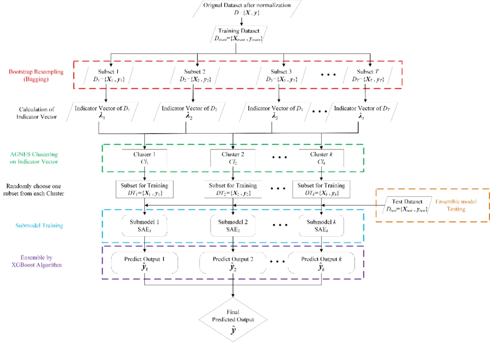
Figure 3:Structure diagram of the proposed method

3.1 Construction and selection of subsets

Assume an original datasetD={X,y} ,whereX∈Rn×m,andy∈Rn×1.After data normalization,the training and test datasets are divided and denoted asDtrain={Xtrain,ytrain} andDtest={X test,ytest} ,respectively,whereXtrain∈Rp×m,Xtest∈Rq×m,ytrain∈Rp×1,andytest∈Rq×1.In the initial construction stage,Tsubsample sets are generated onDtrainthrough the bagging algorithm denoted asDbagging={D1,D2,...,DT},whereDt= {X t,yt},t∈[1,T],Xt∈Rp×m,andyt∈Rp×1.Then,the indicator vector ofXtand the indicator vector set ofDbaggingdenoted as below equations are achieved using Eqs.(6),(7),and (8):

Subsequently,θis clustered through the AGNES algorithm.The AGNES algorithm typically merges clusters with large similarity by measuring the Euclidean distance,as mentioned in Section 2.2.Conversely,clusters with small similarities are not amalgamated.This condition ensures that the indicator vectors within the same cluster are nearly similar.The statistical significance of the indicator vector is to represent the distribution of samples.Consequently,the indicator vectors in the same cluster represent that these subsample sets in the same cluster have a similar distribution.The diversity of these subsets can be viewed similarly.By contrast,the sample subsets between different clusters have a large distance and can be regarded as having a large difference.The indicator vector does not contain the distribution oftrainybecause the diversity of subsample sets placed in the training submodels is focused.

3.2 Construction and training of all submodels

Considering that the threshold increases in a certain step size,the final clustering result is determined on the basis of the number of clusters that decreases the fastest corresponding with the threshold.kclusters denoted asC={Cl1,Cl2,...,Clk} are obtained,wherek＜T.In accordance with the foregoing description,kclusters indicatekkinds of diversity amongDbagging.Thus,one subsample set is randomly selected inClkas the training dataset of the submodel.In particular,kclusters determine that the number of SAE submodels isk.

Suppose that the selected sample subsets for training from all clusters are denoted asDT={DT1,DT2,...,DTk}.Thelth (l∈ [1,k])SAE submodel denoted as SAElusesDTlsubset for unsupervised pretraining and supervised fine-tuning.The adjustable parameters,such as the nodes of each layer in each SAE submodel,are the same.The trained SAE submodel is stored to complete the final integration phase.

3.3 Integration of trained submodels

We focus on the integrated method of all submodels to ensure the final prediction precision of the ensemble model.Following the training process,Dtrain={Xtrain,ytrain} is placed into all trained SAEs to achieve the predicted output of a training dataset expressed as.Subsequently,the optimal ensemble method is obtained by treatingas the training data andytrainas the labeled data for the XGBoost algorithm.Dtest={Xtest,ytest} is placed into each submodel during the testing phase to obtain the predicted output of the submodel denoted as.The final predicted output ofDtest={X test,ytest} is calculated using the trained ensemble model denoted as.

Furthermore,the advantages of the three main factors of integrated modeling are maximized in the three steps of our algorithm.During the construction and selection of subsets,the clustering on the indicator vectors can divide the subsample sets with the largest diversity to the optimal possible extent.During the training of all submodels,SAE improves the prediction accuracy of each submodel given the powerful abilities of fitting and regression prediction of deep learning.The involvement of layer-wise greedy pretraining and fine-tuning can effectively obtain the global optimal solution.During the integration phase,the XGBoost algorithm develops an excellent integration capability to outperform the entire ensemble model.For clarity and concise description,the procedure of our proposed method is presented in Algorithm 1.

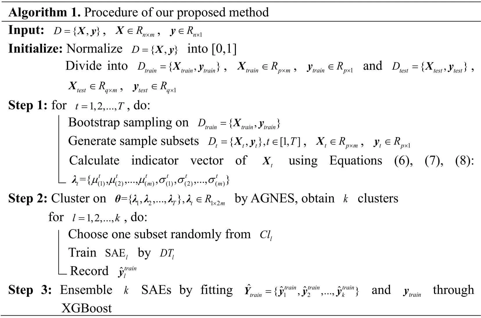
Algorithm 1.Procedure of our proposed method Input:{ ,}X ,1nR ×∈y Initialize:Normalize { ,}D= X y ,n mR ×∈D= X y into [0,1] Divide into { ,}D = X y ,train p mR ×∈train train train X ,1 y and { ,}train pR ×∈D = X y ,test test test X ,1 y Step 1:for 1,2,...,t T test q mR ×∈test qR ×∈= ,do:Bootstrap sampling on { ,}D = X y Generate sample subsets { ,},[1,]train train train y Calculate indicator vector of tX using Equations (6),(7),(8):D= ∈t t t X y ,t p mR ×∈t T X ,1 t pR ×∈λ t t t t t t t m m={ ,,...,,,,...,}µ µ µ σ σ σ(1)(2)( )(1)(2)( )Step 2:Cluster on 1 2 1 2={ ,,...,},θ λ λ λ λ by AGNES,obtain k clusters for 1,2,...,l k T t mR×∈= ,do:Choose one subset randomly from lCl Train SAEl by lDT Record ˆtrain y Step 3:Ensemble k SAEs by fitting 1 2 l ˆ ˆ ˆ ˆ{ ,,...,}Y y y y and trainy through XGBoost train train train train k =

3.4 Model evaluation index

To evaluate the aforementioned model quantitatively,three indicators,namely,root MSE (RMSE),Pearson correlation coefficient (r),and regression index (R2),are used.Three performance indices are defined as

whereexpresses the predicted output of the model,andcorrespond to

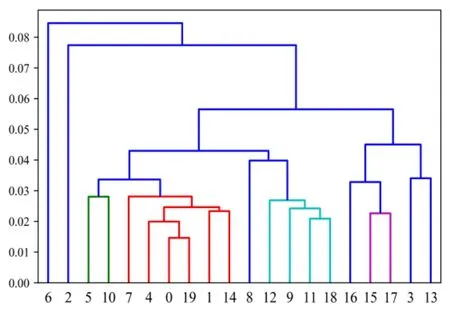
Figure 4:Plot of the AGNES algorithm for BHP clustering (X-axis:Subset Number;Y-axis:Threshold)

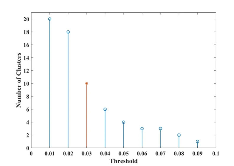
Figure 5:Cluster numbers vary with threshold (BHP)

Table 1:Clustering results on BHP (Threshold=0.03)

4 Experiments and results

In this section,three machine learning benchmark datasets and atmospheric column naphtha dry point (NDP)dataset from the practical industrial process are imported to illustrate the performance of our proposed method.All simulation programs are written in Python and run on a computer with an Intel Core i5-4590 (3.3 GHz)processor and 4 GB RAM.Our analysis and discussion are included.

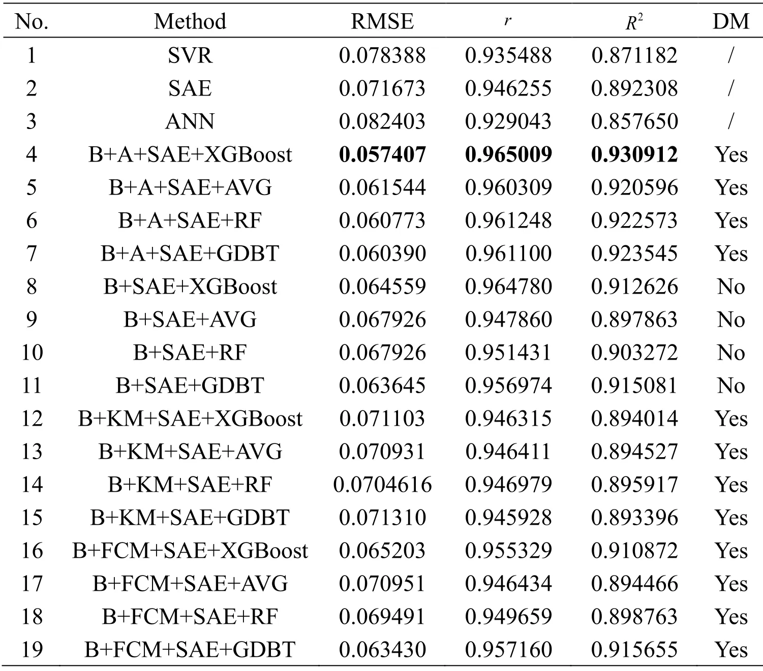
Table 2:RMSE,r,and R2 results of BHP with different models

4.1 Boston house price (BHP)dataset

BHP dataset,which is provided by the scikit-learn library in Python,contains 13 input attributes and 1 output attribute with a total of 506 samples.The description of this dataset can be found in Du et al.[Du,Sun,Cao et al.(2018)].After random disruption,the number of training and test datasets are 404 and 102,respectively.A total of 20 subsets (numbered from 0 to 19)are achieved through the bagging algorithm.The AGNES algorithm clustering of subsets is demonstrated in Fig.4.The step size is set to 0.01.The number of clusters is reduced to maximum extent when the threshold is increased from 0.02 to 0.03.Thus,0.03 is set as the threshold.Fig.5 exhibits the change in the number of clusters with an increase in the threshold.The comparison of Figs.4 and 5 denotes that 20 subsamples gather 10 classes,as displayed in Tab.1.In accordance with the clustering results presented in Fig.4,the number of randomly selected subsample sets from each cluster is written in bold.

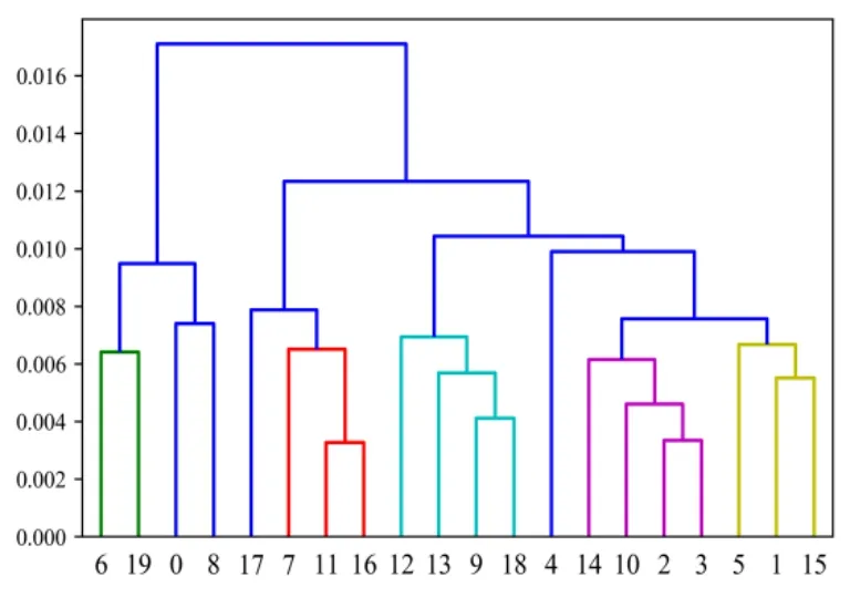
Figure 6:Plot of the AGNES algorithm for CHP clustering (X-axis:Subset Number;Y-axis:Threshold)

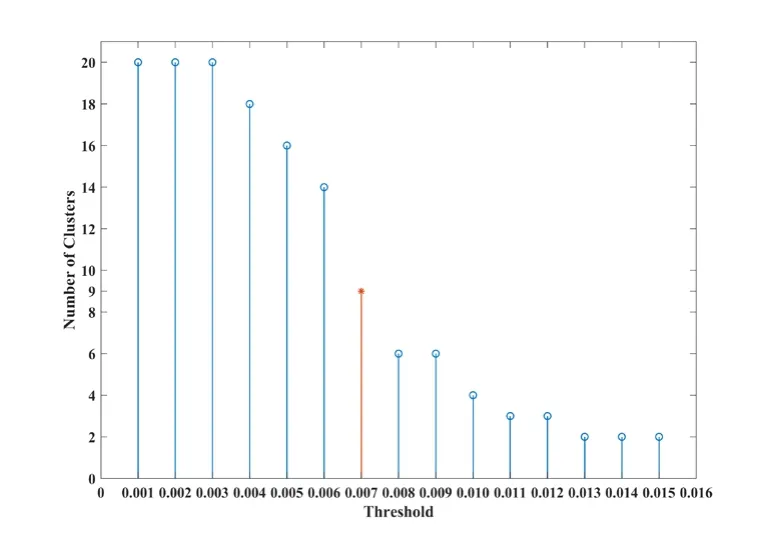
Figure 7:Cluster numbers vary with threshold (CHP)

Table 3:Clustering results on CHP (Threshold=0.007)

All the numbers of the three nodes in the hidden layer of AEs in SAE submodels are 10,7,and 4.Three single prediction models,namely,SAE,SVR,and ANN,without the bagging algorithm and three other ensemble methods,namely,scilicet simple average (AVG),RF,and GDBT,are imported for comparison.To compare the performance of other clustering algorithms through our proposed approach,we use K-means (KM)and fuzzy C-means (FCM)clustering methods to cluster our proposed indicator vectors in parallel experiments.We import Silhouette Coefficient (SC)and fuzzy partition coefficient (FPC)as the indicators to determine the optimal number of clusters for KM and FCM,respectively.The number of clusters,which changes from 2 to 19,corresponding to the maximum value of SC or FPC is the last option.Such methods are equally applied to four datasets.The nodes in the hidden layer in ANN and all AEs in the SAE are set to 10,7,and 4 as well.In SVR,the optimal radial basis function is 1 (σ= 1).The four integrated models use the same input subsample sets to ensure the feasibility of the experiment.The number of trees and max depth parameters are all set to 30 and 4 in XGBoost,respectively.The learning rate of XGBoost is 0.1.

Moreover,the ensemble modeling method without adding the diversity measurement (DM)directly places the subsets generated by bagging into the submodels for training to reflect the importance of DM in our proposed method for improved prediction effect.In particular,the first 10 subsets numbered from 0 to 9 previously generated through the bagging algorithm are directly used for model comparison because the number of submodels is 10.In the comparison experiments,the parameter settings of all models are the same.Under the interference of their respective indicators,the optimal clustering results of KM and FCM are 2 and 16 clusters,correspondingly.Tab.2 demonstrates all parallel experiments on BHP,and the optimal results are written in bold.“A” indicates AGNES,“B” denotes bagging,and “DM” is the abbreviation of diversity measurement.The last column indicates whether or not the process of clustering with the indicator vector to select the subsamples with the greatest diversity is added.

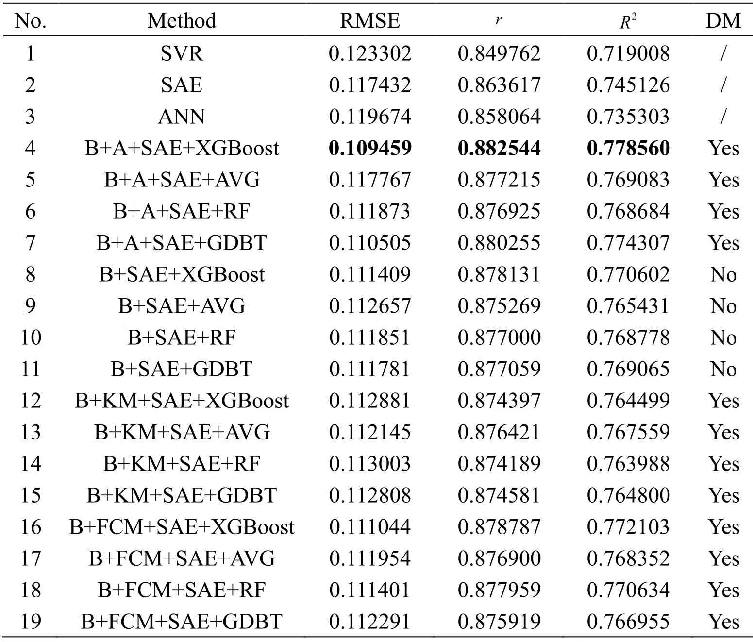
Table 4:RMSE,r,and R2 results of CHP with different models

4.2 California house price (CHP)dataset

CHP dataset,which is supported by the scikit-learn library in Python,consists of 8 independent variables and 1 dependent variable with a total of 20640 samples.A detailed description of CHP can be found in Pace et al.[Pace and Barry (1997)].After normalization,16512 samples are used as the training dataset,and 4128 samples are used as the test dataset.The clustering results are plotted in Figs.6 and 7.These results indicate that 20 subsets through bagging containing 9 subsample sets have large differences.Tab.3 provides the specific clustering results of these subsets from CHP.The hidden nodes of AEs are 6,4,and 3.Radial basis function is applied to SVR ( =1σ).The parameter settings and experiment procedures are the same as mentioned in Section 4.1.The number of trees,max depth parameters,and learning rate are set to 30,3,and 0.2,correspondingly,in XGBoost.The optimal clustering results of KM and FCM are 2 and 14,respectively.Tab.4 summarizes the prediction results of different models for CHP datasets.

4.3 Concrete compressive strength (CCS)dataset

CCS dataset is composed of 8 input attributes and 1 output attribute with a total of 1030 samples and can be obtained on the website:http://archive.ics.uci.edu/ml/datasets/Concrete+Compressive+Strength from UCI Machine Learning Repository.All the meanings of input data can be found in Yeh [Yeh (2006)].The number of training and test datasets are 824 and 206,respectively.In Figs.8 and 9,13 classes are gathered,as listed in Tab.5 in detail.Three nodes in the hidden layer of ANN,SAE,and SAE submodels are set to 6,4,and 3.The radial basis function is adopted to SVR ( =1σ).The parameters of XGBoost are set in the same manner:The number of trees is set to 2000,max depth is set to 3,and the learning rate is 0.1.The optimal partitioning results of KM and FCM are two clusters.The same experimental process functions on the CCS dataset.The obtained results are presented in Tab.6.

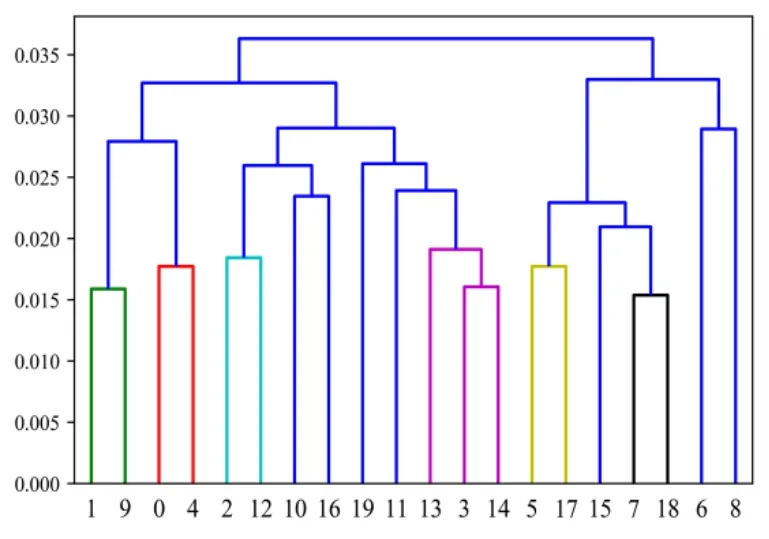
Figure 8:Plot of the AGNES algorithm for CCS clustering (X-axis:Subset Number;Y-axis:Threshold)

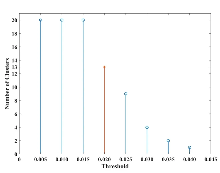
Figure 9:Cluster numbers vary with threshold (CCS)

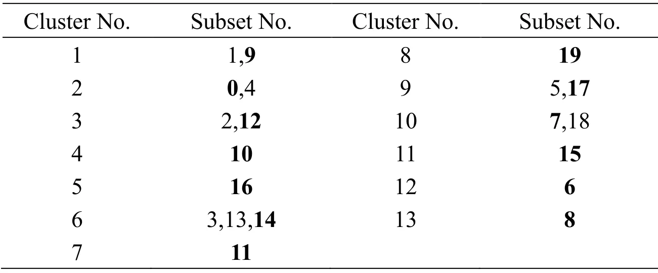
Table 5:Clustering results on CCS (Threshold=0.020)

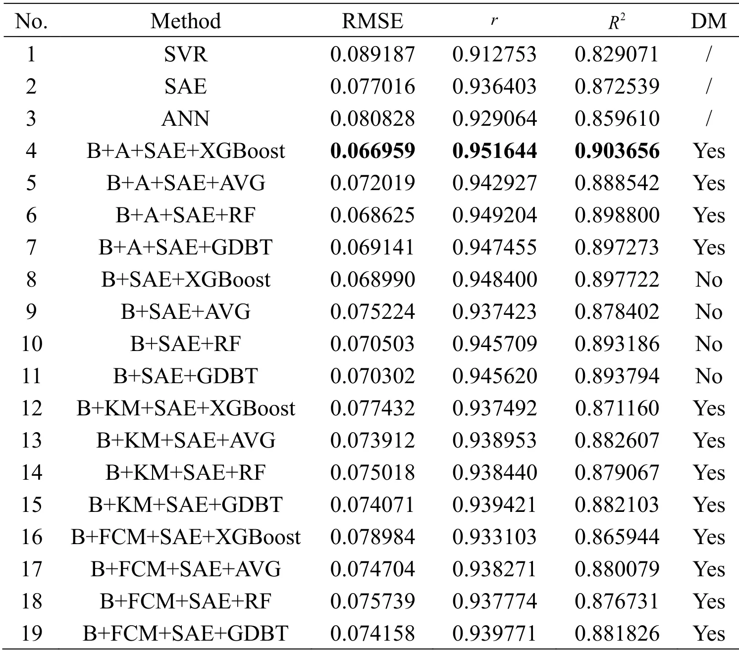
Table 6:RMSE,r,and R2 results of CCS with different models

4.4 Atmospheric column NDP dataset

We apply the proposed algorithm to industrial atmospheric tower modeling to predict dry point temperatures.Atmospheric column NDP dataset is collected from the practical industrial process of a chemical plant.In this experiment,16 input controllable variables and 1 output variable with a total of 150 samples are used.The specific meaning and explanation of each variable are mentioned in Wang et al.[Wang and Yan (2019)].The training and test datasets are divided into 120 and 30,respectively.

After the same clustering on the 20 subsample sets generated through the Bagging algorithm (Figs.10 and 11),13 subsets with significant diversity are obtained,as listed in Tab.7.The simulation experiment on NDP is conducted in the same manner.However,the data from the chemical plant cause large noises in the sample,thereby making the regression effect poor.To quantify the model performance visually,we use maximal absolute relative error (MARE),rather thanR2,as the evaluation index.The calculation of MARE,which expresses the poor results of model prediction accuracy after antinormalization,is formulated as

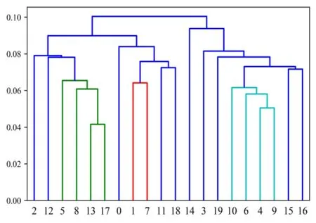
Figure 10:Plot of the AGNES algorithm for NDP clustering (X-axis:Subset Number;Y-axis:Threshold)

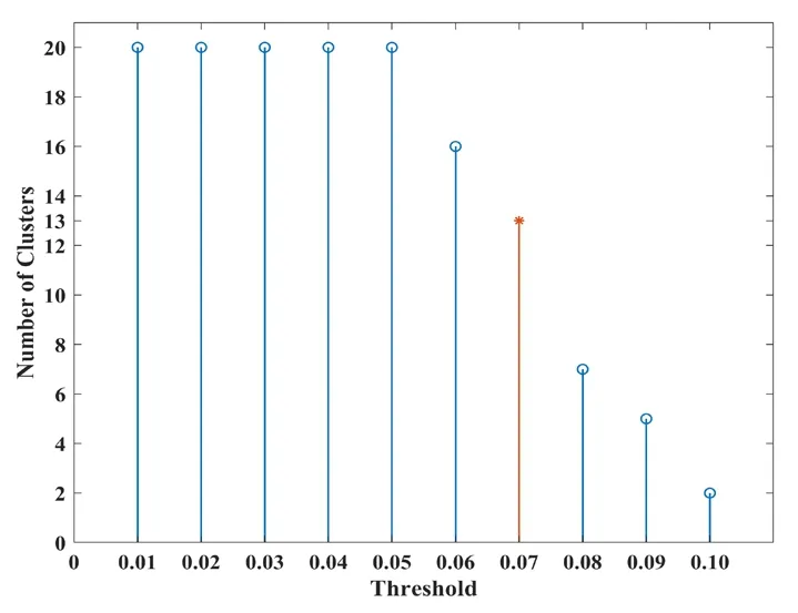
Figure 11:Cluster numbers vary with threshold (NDP)

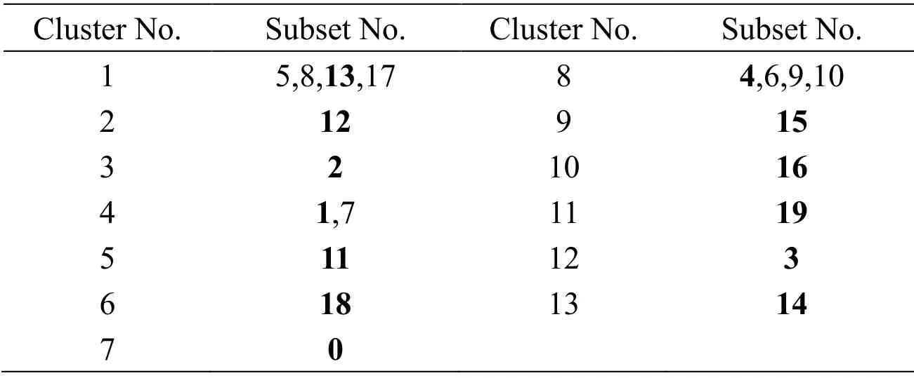
Table 7:Clustering results on NDP (Threshold=0.07)

The hidden nodes in all neural network algorithms are set to 10,7,and 4.The optimal Gaussian kernel function width is 1 ( =1σ).Moreover,the parameters of XGBoost are changed:the number of trees is 200,and the max depth is set to 4.The learning rate of XGBoost is altered to 0.2.Under the SC and FPC indicators,KM and FCM are clustered into two categories as the optimal result.Various algorithm modeling experiment results are summarized in Tab.8.“PI” represents the performance increase in the MARE.The column named “Performance Improved” indicates the increase in the performance of the MARE relative to the model.

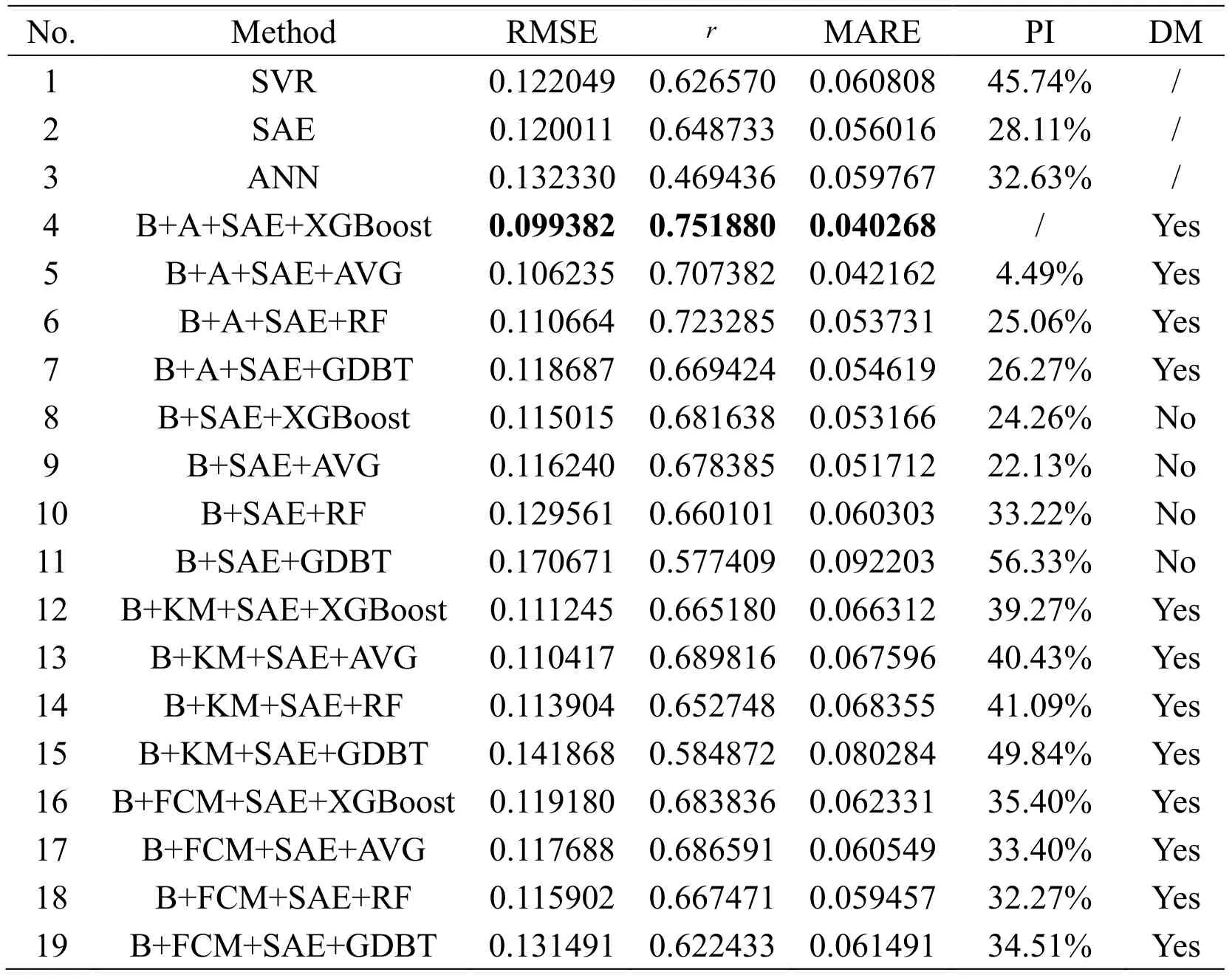
Table 8:RMSE,r,and MARE results of NDP with different models

4.5 Analysis and discussion

The conclusions based on the results of the experiments on four datasets are summarized as follows:

1)Considering the advantages of ensemble models,we compare the different prediction effects of three single models and four integrated models in 19 parallel experiments using the same dataset.Except for some experiments,such as No.8 in Tab.8,the effects of four ensemble models are superior to the single models with a low prediction error in each dataset,thereby demonstrating the superiority of the ensemble model caused by the bagging algorithm.The integrated model can train some sample points that are difficult to predict multiple times,thus compensating the defects in some sample points that may have large prediction errors in a single model,overcoming the overfitting caused by a single model,and reducing the RMSE when testing the ensemble model.

2)In terms of the accuracy of submodels,as presented in Nos.1,2,and 3 in Tabs.2,4,6,and 8,we can infer that SAE shows the optimal prediction results among the three single models considering its advantages caused by deep learning mechanism.The use of SAE as a submodel in the integrated model significantly affects and improves the final prediction accuracy of the final ensemble model.The high accuracy of the submodel indicates an improved integration effect.

3)For the diversity improvement of subsets,the intervention of DM improves the overall prediction accuracy of the model when the integrated model is used on the basis of the comparison of Experiment Nos.4-7 with Nos.8-11 in Tabs.2,4,6,and 8.Furthermore,we can conclude that ensemble models with the DM mechanism measured by the indicator vector significantly increase the diversity of subsamples,thereby allowing the integrated model to achieve high prediction accuracy.The increase in the diversity of subsample sets helps the submodel to learn a rich sample distribution of the original dataset.Thus,the integrated model exhibits a lower RMSE or MARE and higherrandR2than the single model.

4)For the ensemble method,from Experiment Nos.4-7 or Nos.8-11 in Tabs.2,4,6,and 8,the XGBoost ensemble algorithm embodies its powerful integration ability,and the prediction accuracy and regression effect are optimal whether the DM is imported or not.This condition confirms that XGBoost exhibits its extraordinary ensemble capabilities when the submodels are all the same.Although in some cases,such as in Experiment Nos.6 and 7 in Tab.6,therandR2values are slightly lower than the predictions of our proposed model,and the RMSE of our model can be significantly reduced.In addition,the Bagging+SAE+XGBoost algorithm reaches the optimal in comparison with the three other methods when the same modeling method is adopted without DM.The suboptimal algorithm varies with different datasets.However,by comparing Experiment Nos.1-3 with Nos.12-19 in Tabs.2,4,6,and 8,the integration capability of XGBoost is worse than the simple average and slightly better than the single model when the number of submodels is 2.This condition is due to the ensemble effect of XGBoost is correlated with the number of submodels.In Experiment Nos.16-19 in Tabs.2 and 4,the ensemble effect of XGBoost is outstanding,especially on other clustering methods,because the numbers of submodels are 16 and 14.

5)In our model,the AGNES clustering method is irreplaceable.The comparison of Experiment Nos.4-7 and 12-15 with Nos.16-19 displayed in Tabs.2,4,6,and 8 denotes that the clustering results through KM are all two in the four datasets.The number of clusters is small in which the diversity of each subsample dataset cannot be distinguished well,thus leading to the ensemble model obtained through the KM algorithm,and its performance is slightly better than a single model.By contrast,FCM provides the optimal cluster numbers of 16 and 14 in BHP and CHP datasets,correspondingly.Numerous clusters show that nearly all subsample datasets are diverse,thereby resulting in repeated training of some sample subsets with the same distribution.Redundant information directly interferes with the precision of prediction during the ensemble process.However,the prediction accuracy of the final ensemble model using FCM is better than the model using KM clustering and the integration model without adding DM but all worse than the ensemble model of the AGNES clustering method in the BHP and CHP datasets given the increase in the number of submodels and DM.However,the precision effect of the integrated model using FCM clustering or the integrated model using KM clustering is nearly the same in the CCS and NDP datasets when the results of clustering are consistent.Moreover,KM and FCM are required to define the number of clusters and some parameters in advance and calculate the index based on the division result to find the optimal solution,thereby significantly increasing calculation time and computational complexity.In our proposed method,only the step size is required,and the number of clusters is determined by the change in step size.In particular,the number of clusters is adaptively selected in AGNES without calculating additional indicators.This mechanism reduces computational costs,and the number of clusters is moderate.

6)In the BHP and CHP datasets,our methods can significantly reduce the RMSE of test data while increasingrandR2under the same training and test datasets.Experiment Nos.3 and 4 listed in Tab.2 indicate that the RMSE can be reduced from 0.082403 to 0.057407.For the CHP dataset,although the improvement effect ofR2is not evident,our algorithm can reduce the RMSE to less than 0.11 in the case where the RMSE is nearly difficult to reduce.

7)For the CCS dataset,our approach is the only model to increaseR2from approximately 0.8 for a single model to more than 0.9.

8)For the NDP dataset,our method significantly improvesrunder large noise.Simultaneously,the performance of the MARE can be increased to 56.33% for the sample with the largest prediction error.The improvement in MARE performance marks a reduction in prediction error.This condition indicates that our proposed algorithm is the only model that reduces the RMSE of test dataset to less than 0.1.

5 Conclusion

In this study,a novel ensemble modeling method is proposed to overcome three key issues in integrating submodels.These key issues are increasing the accuracy of submodels,improving the diversity of subsets,and selecting the optimal ensemble method.First,the indicator vector and AGNES algorithm simplify the classification of the subsamples with the utmost diversity generated through bagging.Second,in comparison with traditional machine learning submodels,SAE,a deep learning algorithm,is introduced to improve the prediction accuracy of each submodel.Finally,the XGBoost integration capability is used as the optimal ensemble method to fit the nonlinear relationship between various submodels.A total of 19 sets of parallel experiments are conducted in each dataset to highlight the advantages of our algorithm.All results validate that our proposed algorithm outperforms other single or ensemble models for the benchmark datasets and practical industrial dataset.Considering that the ensemble model can effectively improve the robustness and limitations of overfitting caused by a single model,the proposed method can be applied to pattern recognition for classification problems in the future.

Acknowledgement:The authors are grateful for the support of National Natural Science Foundation of China (21878081),Fundamental Research Funds for the Central Universities under Grant of China (222201717006),and the Program of Introducing Talents of Discipline to Universities (the 111 Project)under Grant B17017.