The Exact Inference of Beta Process and Beta Bernoulli Process From Finite Observations

Yang Cheng,Dehua Li, and Wenbin Jiang

Abstract: Beta Process is a typical nonparametric Bayesian model.and the Beta Bernoulli Process provides a Bayesian nonparametric prior for models involving collections of binary valued features.Some previous studies considered the Beta Process inference problem by giving the Stick-Breaking sampling method.This paper focuses on analyzing the form of precise probability distribution based on a Stick-Breaking approach,that is,the joint probability distribution is derived from any finite number of observable samples:It not only determines the probability distribution function of the Beta Process with finite observation (represented as a group of number between [ ]0,1 ),but also gives the distribution function of the Beta Bernoulli Process with the same finite dimension (represented as a matrix with element value of 0 or,1)by using this distribution as a prior.

Keywords: Beta process,joint distribution,beta Bernoulli process,exact inference.

1 Introduction

Non-parametric Bayesian model is a kind of probability model,and the number of parameters of its probability distribution can increase with the increase of the number of samples [Alqifari and Coolen (2019)].It is one of the most important and complex types of Probability Graph models.Therefore,the inference of Non-parametric Bayesian model has always been an important research direction of probability model [Griffin,Kalli and Steel (2018)],such as variational inference [Yao,Vehtari,Simpson et al.(2018)] and regression analysis [Seo,Wallat,Graepel et al.(2000)].

The Beta Process is a Non-parametric Bayesian model.It is mostly used for Bayesian Nonparametric prior of binary sparse characteristic matrix [Andrea,Stefano and Pietro (2018)].It is widely used in various fields,such as Dictionary learning [Liu,Yu and Sun (2016)],Factor analysis [Andrew,Pu and Sun (2017)],Boltzmann machine learning [Lee and Hong (2016)] and so on.As a Non-parametric Bayesian model,it is almost the preferred prior distribution [Romain,Thibaux and Michael (2007)] for a sequence of any length whose element values are within the interval of ( )0,1 .When the Beta Process is taken as the prior distribution of the Bernoulli Process,the Beta Process is marginalized,and the Beta Bernoulli Process will be obtained.When the second parameter of the marginalized Beta Process is set to 1 ,it will become an Indian Buffet Process (IBP)[Griffiths and Ghahramani (2011)].

At present,Paislry has derived a method of Stick Breaking Construction for complete Beta Process,which has been widely used in Beta Process Factor Analysis [John and Lawrence (2009)].It is useful to study the inference method of Beta Process,which depends on the infinite Bernoulli Process tends to the Poisson Process.Similar methods are used to deduce the infinite sequence of IBP.Teh et al.made new progress in this regard (2007)[Teh,Görür and Ghahramani (2007)],and they derived a Stick Breaking Construction method for the special case of “marginalizing the Beta Process in the Beta Bernoulli Process to generate a single parameter IBP”.The Stick Breaking construction method is an important distribution fitting tool of Non-parametric Bayesian model [Eric and Padhraic (2017)],which is widely used in Dirichlet Process [Antoniak (1974)] and Gamma Process [Acharya,Teffer,Henderson et al.(2015)],etc.

Since it is a supervised learning,the task of this machine learning is based on the observable sample,to reversely deduce the model likelihood function contained in the sample after the sampling method is given [Finale and Shakir (2009)].However,different tasks and different conditions will lead to different observable variables in specific tasks.If the observation variable is not the initial variable but the intermediate variable after the operation of the initial variable,the form of the likelihood function itself will change.Therefore,in practice,it is our core processing task to analyze the likelihood function of variables that are more likely to be the final observation variables in some tasks.

The variational inference [John and Lawrence (2011)] of the Beta Process and the likelihood function [Teh,Görür and Ghahramani (2007)] of the Beta Bernoulli Process in the past were mainly used to build the probability distribution function for the intermediate variables needed to generate the sample algorithm.This way of the construction of a probability distribution function is based on the following three basic hypothesis as constraints.

Above all,because in the Stick Breaking Construction method of the Beta Process,the final observed variables sampled from the Beta Process are generated by function mapping and arithmetic operations on two random variables that obey the other two distributions.Therefore,most of the inference work in the past was to directly establish the joint distribution function on the other two intermediate variables,and the result was that the joint probability distribution function itself did not contain the beta random variables [Teh,Görür and Ghahramani (2007);John and Lawrence (2011)].

Afterwards,when the Beta Process samples are generated by using the Stick Breaking Construction method,it is necessary to model the number of rounds in each sample,and the indicator function is adopted,but it is tedious to directly establish the probability distribution for the indicator function of all samples [John and Lawrence (2011)].

Finally,when samples are generated from the Beta Process through the Stick Breaking Construction method of Beta Process,and as a Bernoulli Process prior to the Bernoulli Process modeling,because it is a list of the product of the observed variables as the parameters of the Bernoulli distribution [John and Aimee (2010)],makes it hard for subsequent integral treatment,need through the sampling method of approximate integral operation,Sampling is also a tedious step.

In this work,we intercept a finite number of random variable observations sampled from a Beta Process,calculate a posteriori Bernoulli Process,and make inferences.Here,we mainly do two things.First,for a high-dimensional sequence consisting of any finite number of real number observations with values between [ ]0,1 ,only the hypothesis generated by sampling from a Beta Process is made,and its probability distribution is directly analyzed and inferred.The second is that for a 0/1 matrix that can have any finite row,and each row can have any finite column,you just make the assumption that you sampled from a Beta Bernoulli process and infer its distribution function.The definition of relevant parameters is similar to that given in [John and Lawrence (2011)].The inference process here can be made without any additional assumptions.The above three restrictions can be relaxed in turn:

Above all,we set up the joint probability distribution function of the Beta Process by taking the Beta random variable itself as the observation variable,and the other random variables as the intermediate variables.In this way,the distribution function of the Beta Process can be directly generated by marginalization.

Furthermore,when we construct the likelihood function,instead of recursing the number of rounds of each sample sequentially,we only focus on the number of rounds of the last sample,so that we can directly construct the joint distribution function of the number of samples in each round at one time.

Finally,we analyze the Beta Process of a finite number of observation samples and use it as a prior distribution to directly calculate the posterior probability of the occurrence of any finite dimensional binary valued matrix,so that the posterior probability can be directly analyzed and calculated.Thus,the possibility of any finite dimensional binary matrix is analyzed directly.

Finite dimensional binary matrices can be used to select factors,such as modeling radar signal data.The radar transmits a set of full-bandwidth spectrum data,thenthsample isxn=[xn1,… ,xnL] ,Lis the sample dimension.The factor analysis model can be used to model the full bandwidth spectrum data.Beta Bernoulli priori is used for the model,thenthfull-bandwidth spectrum data is expressed as,and.Where,Φ represents the Shared factor loading matrix of this set of fullbandwidth spectrum data.Kis the number of factors.The sparse weightis composed of weightand binary allocation variableis the noise variable.Where,it can be seen thatωnis used to represent the weight of,while the binary variableznj∈ {0 ,1} is used to achieve sparse,non-zero only in the position of some column vectors of Φ .Here,for the binary variablezn,we use the Beta Bernoulli Process priors.For the Beta Bernoulli Process priors,we usually use the finite approximation of the Beta Bernoulli Process.Here,however,you can directly use the priors of the Beta Bernoulli Process without approximations.

The rest of this article is organized as follows.The second part through the analysis,provides a preliminary knowledge of the Beta Process and the probability distribution function of the observed variables generated by the Stick Breaking Construction method.In the third part,the inference method of probability distribution function of intermediate variable is given.In the last part,the final likelihood function of the observed variable is given by deduction.Describing likelihood function as efficiently as possible is an important step in machine learning with probability model.

2 The definition of the beta process and stick breaking construction

The Beta Process is a nonparametric Bayesian method,which is used to describe a sequence composed of an infinite number of atoms,in which each atom has a weight,and the weight is subject to a degenerate Beta distribution.

2.1 Beta process definition

LetH0be a non-atomic continuous measure on the space ( Ω,B),andH0( Ω )=γ.γfinite.Leta,bbe two positive scalars.Define a processHKas

WhenK→∞ ,HK→H,whereHis a beta process,namelyH～BP(a,b,H0).

2.2 Stick breaking construction of beta process

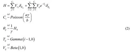
By defining a concept called stick breaking,Paisley et al.[John and Aimee (2010)] clearly proposed a method to build the Beta Process.Stick breaking is a method used to generate discrete probability measure [Ishwaran and James (2001)],which plays an important role in the inference of Non-parametric Bayesian model.For the Beta Process,Paisley et al.[John and Aimee (2010);John,David and Michael (2012)] proposed the following expression method:

2.3 Calculation of edge distribution of kπ

Through the construction of stick breaking concept,Paisley et al.[John and Aimee (2010);John and Michael (2016)] proposed a method that can clearly show the process of the construction of the Beta Process.They divided the probability distribution of elements in the Beta Process into two groups:that isπjis generated in the 1thround,andπjis not generated in the first round of cycles.Paisley et al.[John and Aimee (2010)] calculated the marginal probability distribution of these two types of observations respectively.

Here,whenπkis specified to be generated in theithround,the conditional probability density function ofπkcan be defined as follows:

Wheni= 1 ,the corresponding weight of the atoms in this round follows a Beta distribution,with the first parameter as 1 ,and the second parameter asb.That isVk～Beta(1 ,b)andπk=Vk,Its probability density function is given as,

For other casei＞ 1,we haveπk=Vk e-Tk,andVk～Beta(1 ,b),at the same timeTk～Gamma(i-1,b).Another probability density function can be obtained by calculating the probability distribution of the function of random variables and the probability distribution function of the product of random variables:

where,the intermediate variablew=e-Tkis defined in Eq.( 4 ),and at the same time,iindicates the number of rounds of variableπkoccurrence.

3 Calculation of the joint probability density function of the final observation variables

Previous studies have shown that the number of atoms generated in each round of the stickbreaking construction of Beta Process obeys a Poisson distribution.The stick-breaking construction represented as the superposition of a countable infinite set of independent Poisson processes is useful for further representing the Beta Process.

In order to facilitate the inference,Paisley et al.[John and Aimee (2010)] proposed to use an indicator variablekdto mark the number of rounds in which thethkatom appeared,so as to obtain the formula:

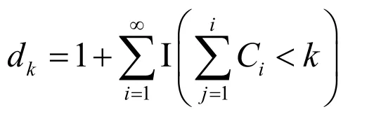
The equationd k=iindicates that thekthatom occurred in t heithround.

3.1 Inference for kd

For gi vendk,we can r econstruct {Ci}i=1.

Figure 1:The relationship between the number of samples contained in each round and variable dk

Given these latent indicator variables,the observation generation process can be rewritten as.By changing the variable,the expression can be redescribed.

When given variabledk≥ 2 ,the variableneeds to be introduced to represent the size of each round.When the corresponding indicator variable of all samples generated in roundjisdk=j,the total quantity isCj.Here means,for example,when all samples generated in round 2 are expressed asdk= 2 ,then the total number of samples in round 2 isC2,and so on.

For given variablesdk≥ 2 ,we use variableto represent the size of each group.

All samples for roundjcorresponding indicator variabledk=j,the total number isCj,this means:All samples for round 2 are represented asdk= 2 ,total quantity of samples in round 2 isC2,and so on.Accordingly,jcan be used to representdkfor sequence analysis of all rounds.

Thus,as shown in Fig.1,the probability of thekthatom being observed in round 1 is:

This is what is shown in the first line frame section of Fig.1.By analogy,the probability ofkthatom being observed in round 2 is:

According to the same reason continue to deduce,can get the final result about the probability of thekthatom appearing in the rounddk.Whendk≥ 3 ,the final result is:

On the other hand,the marginal probability can be viewed as obtained by marginalizing other variables of the joint probability distribution.In this way,the form of joint probability distribution can be obtained through the marginal probability distribution:

Below,we discuss the likelihood terms and prior terms.

The inference processing process of the joint probability distribution of the number of samples generated in each round can be described as follows:

Figure 2:Calculation procedure of probability p ( C1 ,…,Cd k -1,dk )

Here,countis the loop variable.When the loop is complete,the output variable valueMoutis the resultp(C1,…,Cdk-1,dk).

Here,the loop only executesdktimes,and the time complexity is O (dk).Next,we discuss the likelihood term and the prior term.

3.2 Likelihood term

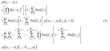
To solve the problem of likelihood term,the integration problem of random variablekdshould be solved first.Here,the conditional probability formula is adopted,and the joint probability can be expanded by the value of variablekd.And then we introduce the joint probability of.From the conditional probability formula,there is:

Eq.(6)proposes a method to realize the joint probability distribution,which represents the observation sequence generated by the Beta Process.We use limited observation (herek)to generate the observation likelihood.here is the joint probability distribution generated by Eq.(5).If we expand and analyze this formula,we can get the integral ofkd.Substitute Eq.(5)into Eq.(6),will get:

3.3 Derivation of conditional probability term

The data is generated byHthrough the Beta Process and expressed in the form of an infinite dimensional vector,with each element between ( )0,1 .The probability distributionis analyzed as follows:this formula is equivalent to the posterior distribution ofπ1,π2,…,π kafter the indicator sequence is given.

3.3.1 Inference fordk=2

Givendkvalue,can reconstruct the {πk}k=1.In other words,ksamples were generated in the first round and the second round,and the sum of the number of samples in the two rounds wask.

Figure 3:the relationship between the value of C1 and variables d k= 2

GivenC1andk,The joint distribution of variablesis:

3.3.2 Inference atdk≥3

Givendk,we can reconstruct {πk}k=1.This means thatksamples are generated in the initialdkrounds,and the sum of the number of samples indkrounds isk,which can be understood as that all samples generated in the firstdk- 1 rounds have been completely observed,while only partial samples have been observed in the last round.

For each round of samples,the corresponding joint probability distribution needs to be defined.So it need to separate the samples from each round.

From the definition of round,we can obtain the elements from thejthround:

Then,given the values ofandk,the joint distribution of variablescan be obtained:

The calculation process of the conditional probabilitycan be described as follows:

Figure 4:Calculation process of conditional probability p (π1 ,…,π k ｜ C1 ,… ,Cd k -1,dk )

Here,,count Iis the loop variable.When the loop is complete,the output variable valueSoutis the result

Fors=1,2,…,ksamplescan be drawni.i.d.from the Beta ProcessBP(a,b,H).

In this way,the joint probability distribution of the final observed variables can be calculated,

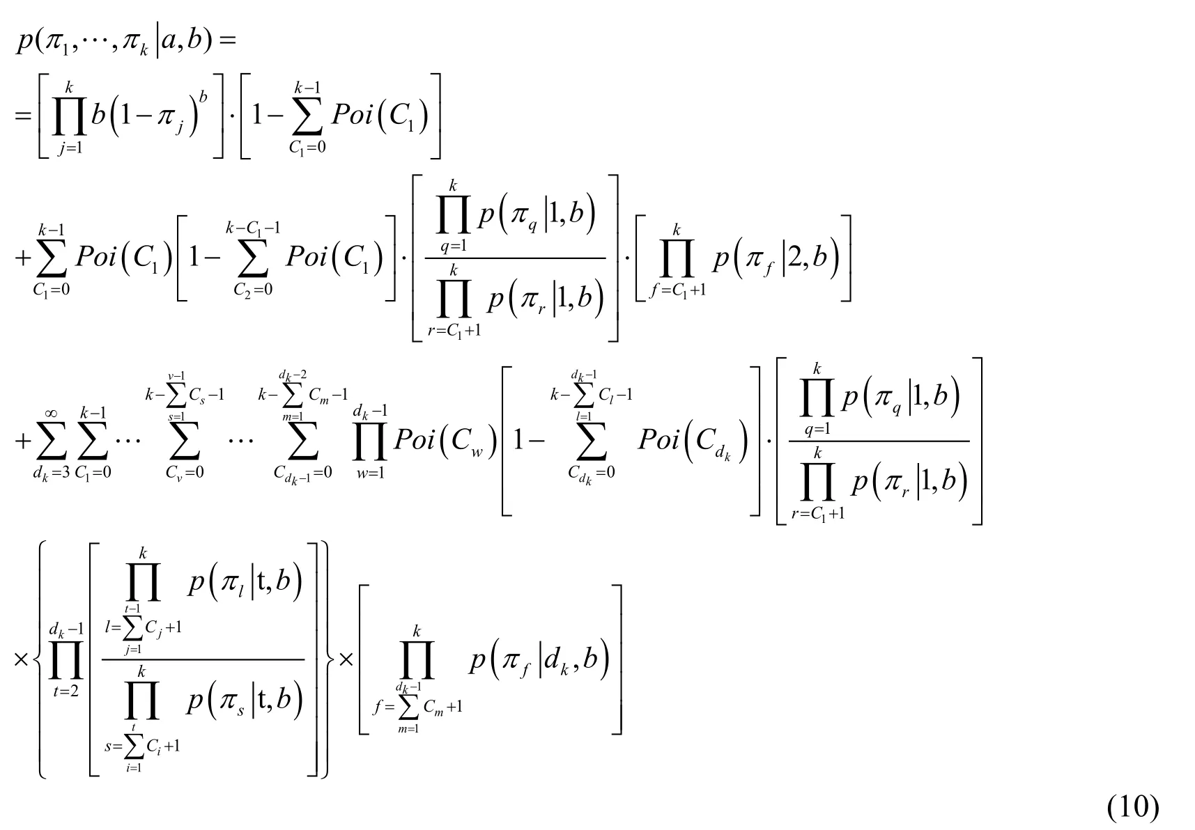
Substituting Eqs.(3)and (4)into Eq.(10),the final precise joint probability distribution function for a finite number of observations of Beta Process is obtained.

Thus,the overall calculation process of the likelihood term can be described as follows:

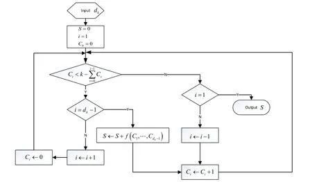
Figure 5:Calculation process of probability p (π 1 ,… ,π k ,dk)

In the calculation process shown in Fig.5,f(C1,… ,Cdk-1)is used to represent the calculation result of multiplyingMoutin Fig.2 andSoutin Fig.4,that is,the joint probability distribution of the observation variable,and the variablethat needs marginalization.The distribution function is:p(π1,…,πk,C1,… ,Cdk-1,dk).The computation time complexity is O (dk).

4 Calculation of the final joint probability distribution function of the observed variables

Datais drawn ...i i dfrom a Beta Process and then via a Bernoulli Process can obtain finite dimensional binary vector form:,Whereigrepresents rowiof matrixZcontainingigcolumn,namely:

This can be represented as ak×gkdimensional binary matrix [Finale,Kurt,Jurgen et al.(2009)].

Figure 6:the relationship between the variables and variables

The sufficient statistics calculated fromare the counts along each dimensionj,so that we have:

wherezijhas been specified to be drawn from a Bernoulli Process with a parameterπi.

Then the Joint probability distribution ofandis subject to:

Here eachπjparameter follows a beta distribution.The joint probability distribution ofcan be calculated by Eq.(10).

By substituting Eqs.(10),(12)into Eq.(13),the exact Joint Probability distribution function of Beta Bernoulli Process for finite observation can be obtained.

Using the above equation,the variablein the intermediate step can be conveniently eliminated by integration,and the result is given in Eq.(15).

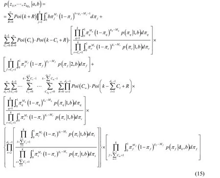
Next,by replacing the distribution of the integral in Eq.(15)by using Eq.(3),we can obtain Eq.(16):

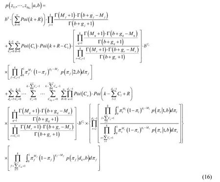
Here,variableRis introduced through the properties of the Poisson distribution:

In order to simplify the following calculation,the calculation form can be appropriately simplified first:

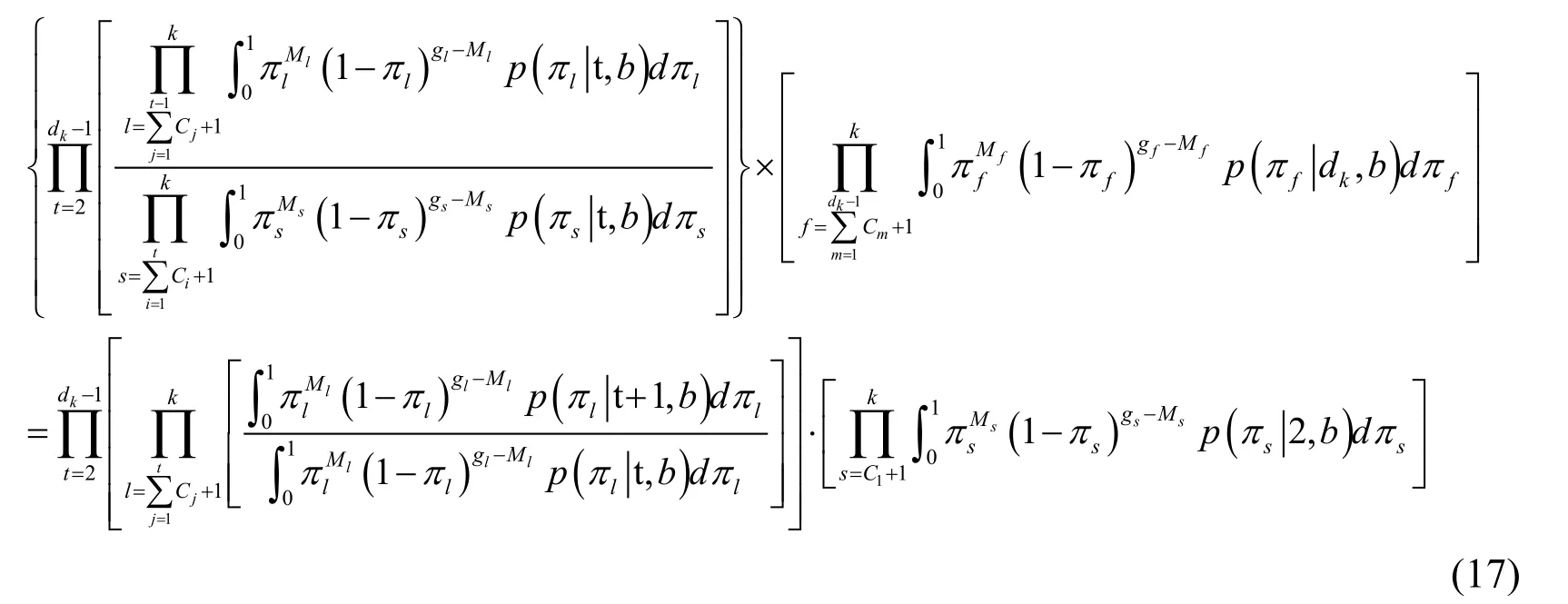
Eq.(17)is a simple shift of the last two terms in Eq.(15).

4.1 Likelihood term for { z k}

Using the conjugate relationship between the Beta Process and the Bernoulli Process,through integral calculation,the following result can be obtained,without loss of generality.The Bernoulli samples produced in roundkdare analyzed here:

In this case,zkwill be used to represent {zk1,… ,zkgk} .and the probability distribution ofπkhas been represented by the Eq.(4).

By Taylor’s expansion,we can obtain the integral of the variableπkanalytically.

Considering series analysis of the middle part of Eq.(18),i.e.,the Taylor expansion of the term,one can find that

Through variable substitution,set,thenR∈ ( 0,1).At the same time have.There are:

The integral result in Eq.(19)can be obtained:

Substituting the calculation results of Eq.(21)into Eq.(18),we can obtain:

This is the likelihood term form of {zk} obtained by inference.

4.1.1 Likelihood term fordk=2

From the above analysis,we now know that since 0 ≤s≤g k-Mk,s≠g k+b,so that haveg k+b-s≠ 0 .Substitutingdk= 2 into Eq.(22),and the following results can be obtained:

4.1.2 Likelihood term fordk≥3

We can use Eq.(22)to calculate the posterior distribution ofzby integrating out the random variablewin Eq.(4)again.In this way,the last integral term of distribution function ofzin Eq.(22)is:

In order to calculate the posterior distribution of a given binary indicator variables,a prior distribution is required.In order to obtain the prior distribution,the following two steps can be performed:

First,variable substitution can be used to calculate the integral.Letu= lnw,and thenw=eu.Therefore,Eq.(24)can be replaced by:

Next we lett=-u(g k+b-s),and then.Substituting these variables into Eq.(25),we can obtain:

4.2 Calculate the proportional term in equation

To calculate the proportional term in Eq.(17),weneed to substitute the result of Eq.(23)into Eq.(17),in this way,we can obtain,

Regarding the integral proportion term in the denominator of Eq.(27),by using the result of Eq.(26),it can be calculated as follows:

Substituting the result of Eq.(28)into Eq.(27),we can produce result:

The Eq.(29)is the final result that we want to get here.

4.3 The final result of the joint probability distribution of

Substitute Eq.(29)into Eq.(17),then the power of constantbin Eq.(17)can be obtained by the following calculation result:

At this time,substitute the results of Eqs.(17),(23),(29)and (30)into Eq.(16),the final calculation result of the variablecan be expressed as follows:

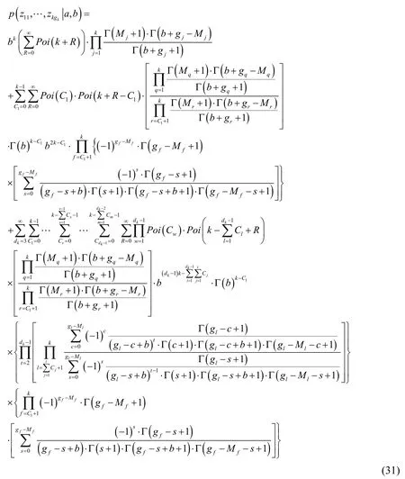
The result obtained from Eq.(31)is the final joint probability distribution function required in this paper.

Here,the calculation of the observed likelihood for each Bernoulli sample is done directly.Thus,the likelihood calculation of each Bernoulli sample is carried out directly.This process can be described as follows:

The calculation result can be analytically generated due to the integration order of beta variableπkand intermediate variablewis exchanged in the function to be integrated,and then Taylor expansion is carried out on the power of (1 -πk)in the exchange result.

The flow chart of the calculation of the final observation variableZin the Beta Bernoulli process is almost the same as that in Fig.4.Since the probabilityin the process described in Figure 4 can be directly used here,due to that the introduction of conditional probability distribution of the observation variable→,and distribution functioncan be analytically calculated by marginalizing variableIπ,i.e.,,then the final resultp(Z)can be obtained.Where,represents theIthrow of matrixZandcountrepresents the number of rounds of theIthvariableπIoccurrence in the Beta Processπ.

5 Beta process factor analysis and the logarithmic likelihood function of the joint probability distribution for beta process

The most commonly used method in machine learning is variational inference,which is often called EM algorithm in parameter estimation.One of its core steps is to calculate the joint probability distribution function of the observed variable and the hidden variable.At the same time,the convexity of the final objective function is guaranteed by taking logarithm of the joint probability distribution function.Therefore,it is one of the most important tasks in machine learning to find the logarithmic likelihood of the joint probability distribution function.For the same reason,the logarithmic likelihood of the joint distribution of Beta Process with finite observations is also calculated below.

The key use of the Beta Process is for Beta Process Factor Analysis [John and Lawrence (2009);John and Lawrence (2011);Ishwaran and James (2001)].Among this,the Bernoulli Process,which takes the Beta Process as a parameter,will be used for factor selection in the set of factors.Therefore,the Factor Analysis of finite observation Beta Process will be discussed in the following part.

5.1 Beta process factor analysis

Beta Process Factor Analysis is mainly described as:Define the matrixand define a set of vectoris the basis vector for the space ofX.Sohas the same dimension as.Here we can set,that is,theXspace is thePdimensional space,.At the same time,we can define a matrixso thatX=Φ (Z◦W)+Eholds.Among them,define a matrix,satisfyAccording to the BPFA definition,we can introduce Beta Bernoulli Process matrixZ,so that:

Through the representation of vector equality,we can get:1≤j≤k.It can be seen here that the random variablezsjindicates whether the component of observationcontains vector,the random variablewsjrepresents the weight of the vectorthat makes up the observation.

The Beta Process Factor Analysis is dealing with:That is,another matrixXis generated from one matrix Φ through vector transformation.Here,elementfπin vectorcorresponds to a vector→ in matrixX.Specifically,GBernoulli 0 1 samplesare generated from a Bernoulli Process with a parameter ofjπ,thenGbasis vectorsneed to be extracted from the corresponding space Φ to constitute

Generally,in the definition of BPFA model,the prior distributions areand

It should be noted that:numerical valueGhere can be arbitrarily large or even tend to infinity.For any countable dimensional space,the description of the space can be realized only by taking out countable basis vectors.Therefore,as long as the number of columns of the matrix Φ is adjusted correspondingly for any countable observation,namely adding irrelevant columns to the matrix,the space of any dimension can be constituted.

The joint probability distribution function can be directly expressed as

According to the definition of distribution function,it can be directly obtained:

In this case,the probability distribution function ofp(Z)can be directly described by Eq.(31).It is usually straightforward to setg i=Gto ∀i.OnlyXis observable here,and the rest are unobservable variables.Theoretically,when the joint probability distribution function is constructed,the work of inference and machine learning can be performed.

5.2 Logarithmic likelihood of the joint probability distribution of beta process

Through Eq.(10),the joint probability distribution function can be directly described.Then,by introducing the intermediate variableand performing the operation,the logarithmic likelihood of the implicit variable can be obtained:

Here,whendk= 2 ,the distribution function of the observation sequence can be directly obtained from Eq.(8)as follows:

Whendk≥ 3,we can calculate the distribution function of the observation sequence from Eq.(9):

From Eqs.(8)and (9),it can be inferred that the above two terms can be uniformly expressed,that is,the conditional distribution of the Beta Process observation sequence can be uniformly expressed as:

At the same time,the joint probability distribution of random variablecan be deduced from Eqs.(5)and (32):

For Poisson Process,introducing random variableRcan be expressed by equivalent substitution:.Then a joint probability distribution function forcan be obtained:

Similarly,through Eq.( 4 ),and variable substitutionT= lnw,the joint distribution function of random variables {π,T} can be obtained:

Here,the range of values for random variables can be limited to 0 ≤Tk≤- lnπk,anddk≥ 2 is required at the same time.

In addition,random variable sequenceis introduced in Eq.(34).The joint probability distribution function ofcan be obtained:

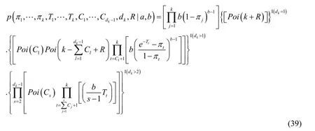
Eq.(36)is the joint probability distribution function form of all random variables that are really needed.It will be calculated below to simplify its representation.

5.2.1 Quotient calculation of{π,T}joint probability

According to Eq.(35),the division of the two terms can be directly calculated.Whens≥ 2,it can be deduced:

When 1s= ,it can be calculated that:

By substituting Eqs.(37)and (38)into Eq.(36),the joint probability distribution function of all required random variables can be obtained:

5.2.2 Logarithmic likelihood of joint probability distribution function

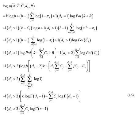
Taking the logarithm of Eq.(39)here,we can deduce:

The structure of joint log-likelihood is analyzed below.

First of all,the coefficient of item logbin Partdk＞ 2 is calculated,and we can get:

With Eq.(41),the calculation ofCjcan be directly completed:

Then,the cumulative calculation of the log (s- 1)items in Partdk＞ 2 can be completed:

For the calculation of the second half of Eq.(43),it can be described as:

By substituting Eq.(44)into Eq.(43),we can obtain:

By substituting Eqs.(41),(42)and (45)into Eq.(40),the following results can be obtained:

Regarding Poisson distribution,it can be calculated as:

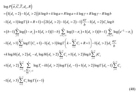
By substituting Eq.(47)into Eq.(46),we can obtain the final conclusion:

Then,by the definition of observation sequence of Beta Bernoulli Process,Formulaandcan be obtained directly.Namely:

Because of the conditional independence between random variables,it can be obtained directly through substitution derivation:

In this case,the logarithmic likelihood function of the final distribution can be obtained by adding the above results:

6 Discussion

Theoretically,the joint probability distribution function must be able to handle any number of observations,and,importantly,the number of actual observations can be arbitrarily large,but not infinite.The method that we have given here is simple and effective in dealing with this problem,because the Nonparametric Bayesian stochastic Process we discussed here does not satisfy the Kolmogorov consistency theorem,so lead to the relationship between observed variables is not independent identically distributed.The distribution function form is much more complicated than the traditional machine learning situation,and the number of unobserved variables has a direct impact on the form of the distribution function.The method proposed here eliminates the information irrelevant to observations and thus gives the general form of any finite number of observations.

We have obtained several results of this idea through the Stick-Breaking structure proposed by Paisley et al.[Paisley and Zaas (2010)]:including the more general construction of finite observation and the new type of joint probability distribution function for Stick-Breaking Beta Processes,which indicates that the Beta Process is the superposition of a Poisson Process countable set and used as a priori of Bernoulli Process.Finally,a finite observation of a 0/1 matrix is completed.

In the future,we will extend the proposed method and use variational inference method to solve the problem that the accurate estimation of marginal distribution is too complex,so as to be applicable to the machine learning task of approximate parameter estimation of Beta Process and Beta Bernoulli Process.We will also explore some approximate inference models of distribution functions of Non-parametric process variables,hoping to obtain better and simplified performance by means of variational inference method.These similar methods can also be used for Gamma Processes [Anirban and Brian (2015)] and Gamma Poisson Processes [Michalis and Titsias (2007)].This is the next step of our consideration.Regression analysis is one of the main research directions in the field of machine learning.At present,Gaussian Process Regression is the main regression method when stochastic process is used as the tool.Among them,Kalman Filter is the most widely used field in Gaussian Process Regression.Based on the same idea,because for the Beta Process,when the joint probability distribution function is given,the conditional probability can be calculated according to the Bayesian formula and the regression analysis can be carried out theoretically.Therefore,the regression analysis of Beta Process is also one of the directions to be considered in the next step.

The idea described above can be also used in the context of Gamma Processes similar to Beta Processes,so our results also contribute to the establishment of a general Nonparametric Bayesian inference mechanism.

A more common variant of the Beta Bernouilli Process is the Indian Buffet Process (IBP),which learns the number of features included in the model from the observed data,thus allowing the model to interpret the data more accurately.The Non-parametric Bayesian model based on IBP can automatically learn the implicit features,and can in a scalable way to determine the number of features.Therefore,in theory,better prediction performance can be achieved.In practical applications,the 0/1 output of the Beta Bernouilli Process is generally used to describe the relationship between entities.In the sample matrix of the Beta Bernoulli Process,a specific entity is described by a set of binary features,and then the features are obtained from the observations.And try to infer the features.The sample matrix value of the Beta Bernoulli Process can be used as a basis for determining whether the entities are related.If the weight is attached to the 0/1 output of the Beta Bernouilli Process at the same time,the strength of the influence between the entities can be added while describing the correlation between the entities.

Since the distribution of the Beta Bernouilli Process is long-tailed,and the distribution functions for each round generated by the Beta Process Stick Breaking do not necessarily have the same attenuation trend as the power-rate distribution,resulting in the model being basically sufficient to describe the entity possessing any number of features.The general Beta Bernouilli Process describes the probability distribution,which can be used to describe the relationships between entities,and the relationships are not necessarily symmetric.This asymmetry relationship can be applied to some important issues such as social network connection prediction.Connection prediction is an important issue in social network modeling [Miller,Michael and Thomas (2009)].Here,it can be assumed that the link probability from one node to another node is determined by the combined effect of pairwise feature interactions.If a weight is added to the 0/1 sample matrix of the Beta Bernouilli Process,and the positive weight corresponds to the probability of high correlation,while the negative weight corresponds to the probability of low correlation,and the zero weight indicates that there is no correlation between the two features,then the representation ability of the model will be greatly improved,and the influence relationship between nodes will have stronger performance.

The relationship between entities can be simplified.The simplified symmetric relationship is used to learn a complete symmetric weight matrix.The symmetric Beta Bernouilli Process model can also be used to describe the co-authorship relationship judgment in text mining,because the co-authorship relationship is symmetric [Teh,Jordan,Beal et al.(2006)].

Currently,IBP Process with multiple levels proposed by the academia has been applied in Deep Learning.It is used to learn the structure of Deep Belief Network,including the number of layers of neurons,the number of neurons in each layer,and the connection structure of neurons between layers [Adams,Hanna and Zoubin (2010)].

In this paper,the exact analytical form of probability distribution function of finite arbitrary dimension is directly analyzed for Beta Bernouilli Process,and its properties as the objective function of machine learning are discussed.In the next step of prediction [Miller,Michael and Thomas (2009)] and learning [Adams,Hanna and Zoubin (2010)],it can be directly used as the prior probability distribution function of the discriminant model [Miller,Michael and Thomas (2009)] and substituted into the objective function for parameter optimization.

Since the marginal probability distribution function defined here is accurate,the calculation process of parameter optimization can be carried out based on demand,or we can directly optimize the precise distribution of marginal probability,or choose sampling [Miller,Michael and Thomas (2009)] and variational inference to make approximate inference to the joint probability distribution function.

In Deep Learning,ideas similarity of Teh et al.[Teh,Jordan,Beal et al.(2006)] can also be used to conduct Deep Learning reasoning by taking the row number and column number of each row of the binary matrix output by the Beta Bernouilli Process as the layer number of multi-layer neural network and the node number of each layer.The two-parameter beta process description adopted in this paper theoretically promotes the model in [Adams,Hanna and Zoubin (2010)],which directly adopted the Indian Buffet Process as the priori of the number of layers and the number of nodes of each layer of Deep Belief Network.

7 Conclusions

Beta Process contains a list of random variables.However,these random variables do not satisfy the stationarity or the global independent increment,so the probability distribution of these random variables has an extremely complex form.The stick breaking construction method is a means to indirectly define the Beta Process by describing the sampling process.Further analyzing and deducing the joint probability distribution of observed samples through the described sampling method is the next step necessary for machine learning.The result presented here is an analytical method for directly calculating the probability distribution of observable variables in Beta Process.Through probability distribution calculation,on the one hand,all intermediate variables are directly marginalized,thus completely eliminating the unobservable information.On the other hand,the observation of Bernoulli Process directly generated by taking Beta Process as a parameter can have the form of analytic probability distribution function.

In the future,we will further extend the derived results and deal with the later steps of machine learning on the Beta Process.