An algorithm to separate wind tunnel background noise from turbulent boundary layer excitation

Xiojin ZHAO, Mingsui YANG, Jie ZHOU, Junmin LEI

a School of Aerospace Engineering, Beijing Institute of Technology, Beijing 100081, China

b AECC Shengyang Engine Research Institute, Shenyang 110015, China

c Department of Mechanical and Aerospace Engineering, Hong Kong University of Science and Technology, Hong Kong, China

KEYWORDS Background noise;Sound source separation;Turbulent boundary layer;Wall pressure fluctuation;Wind tunnel

Abstract Wall pressure fluctuations generated by Turbulent Boundary Layers (TBL) provide a significant contribution in reducing the structural vibration and the aircraft cabin noise. However,it is difficult to evaluate these fluctuations accurately through a wind tunnel test because of the pollution caused by the background noise generated by the jet or the valve of the wind tunnel. In this study, a new technology named Subsection Approaching Method (SAM) is proposed to separate the wall pressure fluctuations from the background noise induced by the jet or the valve for a transonic wind tunnel test. The SAM demonstrates good performance on separating the background noise from the total pressure compared to the other method in this study.The investigation considers the effects of the sound intensity and the decay factor on the sound-source separation. The results show that the SAM can derive wall pressure fluctuations effectively even when the level of background noise is considerably higher than the level of the wall pressure fluctuations caused by the TBL. In addition, the computational precision is also analyzed based on the broad band noise tested in the wind tunnel. Two methods to improve the precision of the computation with the SAM are also suggested:decreasing the loop gain and increasing the sensors for the signal analysis.

1. Introduction

The continual development of jet-engine-powered, wellstreamlined aircraft draws extensive attention to the sound and the vibration induced by the turbulent boundary layer of high-speed airflow. The turbulent boundary layer is responsible for reducing the sound level inside the cabin during the cruise condition,1which is an important index of aviation requirements. To develop effective ways to reduce this sound level, the noise associated with the turbulent boundary layer needs to be reliably predicted.

Reliable wall pressure fluctuations and noise generated by the turbulent boundary layer are usually obtained in wind tunnels.2-6The measured wall pressure fluctuations could be used to validate the CFD simulations7-12and correct wavenumberfrequency models.13-16However, wind tunnel tests of wall pressure fluctuations are not always perfect, and the results are usually contaminated by the background noise in the wind tunnel.

To obtain the signal of interest, the background noise should be separated and deleted from the measured results.

Generally, in a low-speed wind tunnel with the maximum speed not higher than 100 m/s (Mach number Ma ≈0.3),17,18the primary noise source is the fans used to accelerate the airflow. However, in a transonic or supersonic wind tunnel, the background noise is mainly composed of the jet and the valve noise,19-21and the noise generated by slots and the perforated walls of the test chamber.22-24

Some investigators17,18,25-28tried to reduce the effect of background noise on wall pressure fluctuations and aeroacoustic measurement. However, these studies focused more on the measurement of radiated noise and most required a higher SNR (Signal to Noise Ratio) for the signal of interest to remove the background noise with the acoustic array technology.17Meanwhile, the flow speeds involved in these studies17,18,25-28did not exceed 100 m/s (Ma ≈0.3) and the suppression of background noise was mostly achieved with advanced signal processing methods.18,26-28

Ref.23showed that strong background noise still exists in many transonic and supersonic wind tunnels and the pressure fluctuations measured in these wind tunnels could be seriously contaminated by the background noise caused by the jet or the perforated wall.To control the background noise generated by the perforated wall of the test chamber, the perforated wall could be covered with wired screens.23To reduce the effect of the valve noise on the aero-acoustic measurement,a special absorptive structure29could be installed around the test chamber of the wind tunnel. However, the experimental cost would certainly be increased. In addition, some optimization techniques have been proposed to reduce the effect of the background noise through phase array signal processing;however, the algorithm used for the phase-array test cannot directly separate the background noise from the wall pressure fluctuations owing to the special requirement of the array distribution (for example, spiral design) in the phase-array technique.

Hence, this study attempts to develop an algorithm to subtract the component of background noise caused by the jet and the valve in a transonic wind tunnel without using any noise absorptive structure.This technique could be applied to higher flow speeds beyond the range of the applications of traditional phase-array methods. This investigation is inspired by the work of Goldstein30and Sinayoko et al.31To separate these two kinds of pressure fluctuations, Goldstein30suggested in an unbounded turbulent field, the aerodynamic noise be decomposed into non-radiating and radiating components.Then, Sinayoko et al.31separated the radiating acoustic components from the non-radiating components in the nonlinear flow equations using linear convolution filters. The wall pressure fluctuations can be treated as the non-radiating acoustic component and the jet and valve noise belong to the radiating acoustic component according to their forms of production.30,31The method developed here aims at separating the jet and valve noise from the pressure fluctuations in a transonic flow when strong pressure fluctuations are usually induced32over the structure.

The remainder of the paper is organized as follows: Section 2 describes the theoretical model of different sound sources. Result comparisons are presented in Section 3. The final section, Section 4, provides conclusions.

2. Theoretical model

2.1. Sound source model

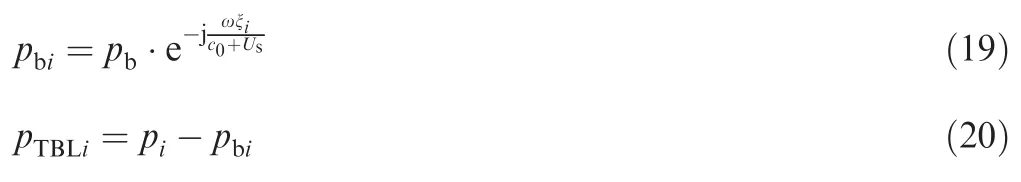
To separate the background noise,the first step is to determine the mathematical expressions for the background noise and the wall pressure fluctuations generated by the turbulent boundary layer.Fig.1 shows a test model fixed in the wind tunnel in the wall pressure fluctuations test. According to the equation of the convection wave, the background noise caused by the jet exit vanes downstream or the valve used for controlling the airflow upstream can be expressed as follows:

where pbω( ) indicates the amplitude of the sound pressure around the test model belonging to the background noise, ω the angular frequency, c0the sound speed in the wind tunnel,Usthe velocity of the local flow and ξxis the variation of the distance along the stream-wise direction. Eq. (1) presents the background noise generated by valves or jets, propagating to the test section of the wind tunnel.It is assumed that the amplitude of the background noise does not decay along the flow direction or around the test model because the coordinates of the sensors installed on the test model change only slightly.

Generally, the wall pressure fluctuations under a TBL can be simulated by wavenumber-frequency spectrum models,such as the Corcos model,32-34Efimtsov model,35,36and Chase model.37These different TBL models are adapted to different situations mostly determined by the inflow speed and the configuration of the test model.The classical Corcos model is only suitable for describing TBLs with low mean flow velocities.However, the extended Corcos model32can cover low-speed,subsonic, and transonic flows passing through a typical covecylinder structure. Hence, to separate the background noise at a transonic flow, which regularly induces serious pressure fluctuations over the structure, the extended Corcos model32is adopted in this study to simulate wall pressure fluctuations.

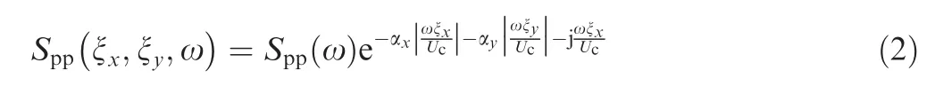
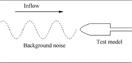
Fig. 1 Test model measured in a wind tunnel.

In the frequency domain, the wall pressure fluctuations described by the classical Corcos model can be expressed as:33,34where Ucindicates the convection velocity, and it is suggested that 0.5U0≤Uc≤0.7U0,38U0is the mean flow velocity;x and y represent the coordinates along the stream-wise and spanwise directions in the model, respectively; ξxand ξyindicate the distances between the two arbitrary points on a plate in stream-wise and span-wise directions, respectively; αxand αyare the decay rates in x and y directions,respectively;Sppindicates the amplitude of the wall pressure fluctuations.

Generally, Eq. (2) is only suitable for describing low-speed flows when pressure gradients are too small to be considered within the TBL. If the incoming flow is in high subsonic or transonic speeds,the extended Corcos model32should be used to simulate the attached flow, and the expression of the extended Corcos model is:

In addition, if the extended Corcos model is used to simulate the separated flow,32Eq. (3) should be modified as:

To describe the shock wave oscillation,32the Corcos model can be expressed in the form of:

Eqs. (3)-(5) show that TBL models always consist of two components, the decay of the amplitude of wall pressure fluctuations and the phase change of the TBL excitations at different points. The expressions of pressure fluctuations under different flow conditions, including the attached flow, the separated flow and the shock wave oscillation can be integrated into a uniform form:

Eq. (6) indicates that the cross-spectral density of the wall pressure fluctuations at two different points on the test model could be expressed in terms of the correlation between the pressures at two arbitrary points:

where pTBLX，ω( ) indicates the variation of the wall pressure fluctuations induced by the TBL over the structure. Although Eq. (7) indicates the correlation in power and Eq. (6) represents the correlation in pressure,both equations present a consistent phase variation as Eq. (7), which can be derived from Eq. (6).

Eqs. (1) and (7) require that the propagation speed of the background noise in the wind tunnel must be different from the speed of the flow convection.Otherwise,serious coherence between the background noise and the wall pressure fluctuations will be generated and the change of phase differences between the two disturbances is eliminated. In this case, the computed phase difference between any two continuous sensors remains constant and it will be impossible to separate the background noise from wall pressure fluctuations by Subsection Approaching Method (SAM). The condition of‘‘c0+Us≠Uc” is the assumption required by the technology used for sound-source separation in this study. However,‘‘c0+Us≠Uc” is always satisfied in this study because c0＞Ucall the time for the transonic flow. In addition,although the proposed method aims at solving the background noise of the transonic flow, its application is not confined to transonic flows. If the condition ‘‘c0+Us≠Uc” is satisfied,sound source separation could be extended to supersonic flows or even hypersonic flows theoretically.

2.2. Sound source separation

Eqs.(1)-(7)show that the background noise and the wall pressure fluctuations generated by the TBL are not coherent when c0+Us≠Uc. Therefore, it is possible to subtract the background noise directly from the compound signal measured in the wind tunnel test.Based on the difference between the propagation velocity of the background noise and the convection velocity of the flow,the SAM is proposed to separate the background noise from wall pressure fluctuations in this study.The background noise propagates at the speed of sound, while the pressure fluctuations induced by the TBL are determined by the convective speed of the inflow.

Wall pressure fluctuations induced by the TBL are usually measured by a sensor array. Fig. 2 shows the sensor array designed for the SAM,in which sensors are arranged in a line.Assume that the pressure signals are collected by the sensors of the array, and they could be expressed as:

where piindicates the pressure-signal collected by the ith sensor,and N is the total number of the sensors used in the array.

At each point,the sound pressure picontains both the pressure induced by the TBL and the background noise.According to Eqs.(1),(7)and(8),the pressure measured at each test point can be represented as:

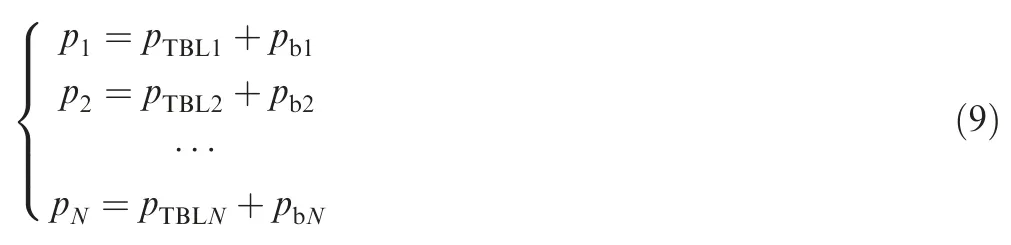
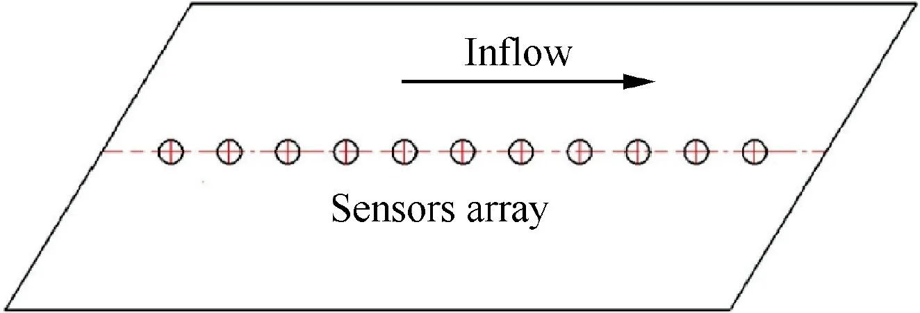
Fig. 2 Sketch of sensor array.

Then the prince s servant brought in the three robes, and when the judges saw the mist-gray one which the princess usually wore, they said, Have this robe embroidered10 with gold and silver, and then it will be your wedding robe.

The SAM is a method based on numerical calculation,and basically, the coherence of wall pressure fluctuations at different test points is used to separate the background noise.According to Eq. (7), though the amplitude of the wall pressure fluctuation at each test point is different,the phase differences between the wall pressure fluctuations at any two successive test points are the same if the sensors are distributed with equidistance. This is the fundamental principle used by the SAM for sound source separation.

The computational flowchart of the SAM is shown in Fig. 3. In using the SAM to separate the noise, the first step is to define the initial variations used to store all the pressure data measured by the sensors and some important parameters required in the computation. The definitions of all the initial variations are listed as follows:

Fig. 3 Subsection approaching method with n subsections.

where ‖ ‖ indicates the modulo, temp0determines the ranges of the amplitudes of the background noise and the wall pressure fluctuations, anddefines the range of the propagating speed of the background noise in the wind tunnel relative to the sound speed.

To avoid the divergence of computation, a loop gain φ is introduced to control the step of computation and‘‘0<φ<1” is suggested to buffer the computation. When n subsections are used for the computation, as presented in Fig.3,the loop gain could choose‘‘φ=1/n”.The step lengths of the amplitude and the velocity can be expressed as‘‘Δp=φ·temp0” and ‘‘ΔUs=φ·U0”, respectively. Then we address the first three sensors:

Through the first step of the computation, the computed background noise and the wall pressure fluctuations are closer to the real values than the initial values defined in Eq.(13). In the second step of computation, the step lengths of the amplitude and the velocity are updated with new variations to improve the precision of the simulated background noise:

In addition, increase one more sensor for the computation of the phase differences between two neighboring sensors:

Define Max=Maximum(abs (ΔPha2，3-ΔPha1，2), abs(ΔPha3，4-ΔPha2，3), ... , abs(ΔPhaN-1，N-ΔPhaN-2，N-1)),ΔPhai，j=Phase()-Phase(),i，j=1，2，···，N, and Max indicates the maximum value when i and j are changed from 1 to n.

Meanwhile, change k and l to find ‘‘Minimum (Max)”.When ‘‘Minimum (Max)” is found, update l and k with lminand kmin, respectively, and stop the computation. Then, the final background noise and the wall pressure fluctuations are the closest to the real values:

where pb=lminΔp+amp, Us=kminΔUs+Pha, and Δp， ΔUsare computed by Eq. (17).

According to the presentation above,the SAM is an asymptotic method based on the numerical computation. An overt merit of the SAM developed is that it could resolve wall pressure fluctuations without knowing the precise information of them,such as their intensity,the decay factor,and the convection velocity, thus it is easier to apply in engineering applications. In addition, although the SAM is derived based on the signal collected by an equi-spaced array, the instrument is not confined to equi-spaced array systems.The reason of using an equi-spaced array here is that it is also used to obtain the pressure distribution along the streamwise direction of the model.

2.3. Precision analysis

The precision of the computation is a vital factor affecting the separation of the wall pressure fluctuations from the background noise.According to the SAM introduced in Section 2.2,the precision of the signal separation is determined by the step lengths of the amplitude and the velocity used in the computation.The expressions of the step length are shown in Eq. (17),which shows that the step lengths of the amplitude and the velocity are both determined by the loop gain φ(0<φ<1)and the number of sensors used to record the raw signals.The larger the step length, the lower the computational precision. Hence, the precision of analyses could be improved in two ways: decreasing the loop gain, or increasing the number of sensors used to collect the raw signals. However, it is uneasy to determine the value N and the loop gain to obtain a best result of sound separation.The more the number of sensors and the smaller the loop gain, the higher the accuracy of the acoustic separation and the longer the iteration time.Sometimes, for small loop gains, the iterative computation of the sound separation is not even convergent. In most cases,the appropriate values N and the loop gain should be determined by the calculations based on the frequency range of interest and the required accuracy.

3. Comparisons of results

Generally,the separation of signals is influenced by many factors, such as the intensities of the wall pressure fluctuations and the background noise, the decay factors of the wall pressure fluctuations, and the analysis frequencies. In this section,these factors are discussed and the proposed method of background noise separation is validated.

3.1. Effects of intensities of wall pressure fluctuations and background noise

Fig. 4 demonstrates that the SAM can accurately separate the wall pressure fluctuations from the background noise when they are at the same level. Unfortunately, the wall pressurefluctuations are sometimes much lower than the background noise. In such cases, the wall pressure fluctuations are almost submerged in the background noise (Fig. 5), and the difficulty in separating this signal from the background noise is considerably increased.Fig.5 presents the results of the sound source separation when the background noise is much larger (ten times of the wall pressure fluctuations) than the wall pressure fluctuations, and pbω( )=10 Pa, pTBLω( )=1 Pa. The results show that the SAM can still separate the wall pressure fluctuations from the background noise even when the wall pressure fluctuations are much lower than the background noise.

Table 1 Coordinates of sensors in array.

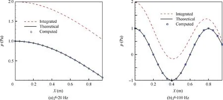
Fig. 4 Comparison of results of sound-source separation with intensities of background noise and wall pressure fluctuations in same level.

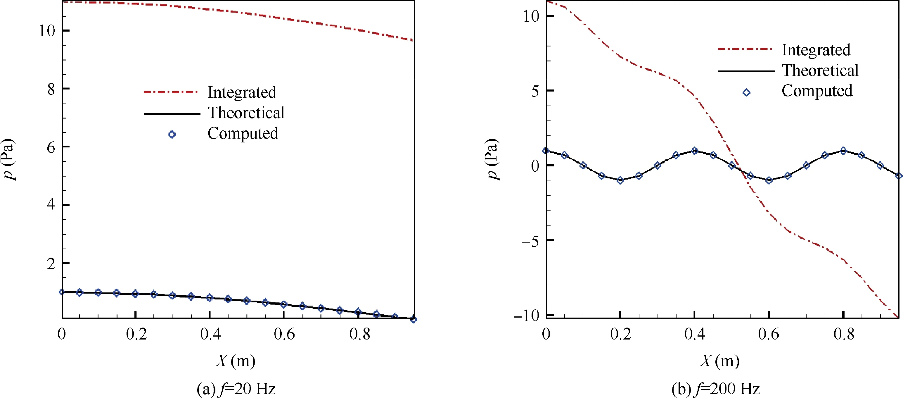
Fig. 5 Comparison of results of sound-source separation with intensities of background noise ten times of wall pressure fluctuations.

3.2. Effects of decay factor

Generally, the amplitude of wall pressure fluctuations varies along the flow direction, as described by the decay factor in Eqs. (4) and (5). Hence, it is necessary to consider the effect of the decay factor on sound-source separation. Fig. 6 shows the results of sound-source separation when the decay factor is considered, and the real parts of the background noise and the wall pressure fluctuations are presented. The decay factor chosen here is 0.5. The integrated sound-source is computed by the method mentioned in Section 3.1 with sound speeds c0=340 m/s, U0=225 m/s, and Uc=0.65 U0. The broken lines in Fig. 6 indicate the integrated pressure signals of the background noise and the wall pressure fluctuations.The solid lines represent the theoretical results of the wall pressure fluctuations,and the diamonds show the results obtained with the SAM.The decay of the wall pressure fluctuations decreases the weighting of the wall pressure fluctuations in the integrated signal (of the background noise and the TBL noise) along the flow direction. As shown in Fig. 6(b), the interested signal has almost decayed to zero after X=0.2 m when the decay coefficients are large. The integrated sound pressure is dominated by the background noise which is presented in the form of a standard sinusoidal wave (Fig. 6(b),) after the interested signal has decayed to zero (X>0.2 m). However, the SAM can still separate the wall pressure fluctuations from the background noise accurately (Fig. 6).

3.3. Broadband signal separation analysis

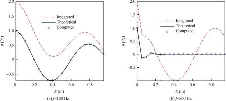
Fig. 6 Comparison of results of sound-source separation with decay factors considered.

Aeroacoustics also deals with broadband noise.To investigate the sound-source separation for broadband noise, a pressure signal measured in the FD-12 wind tunnel(China)is used here to simulate the wall pressure fluctuations generated by the TBL. The pressure signal is measured by a pressure sensor at a Mach number of Ma=0.8 and the measured sound pressure spectrum is shown with a solid line named‘Original'in Fig.7,and SPL indicates sound pressure level. Here, this measured pressure signal is assumed to be an interested signal which needs to be separated from the background noise. To create a noisy environment for the sound-source separation, an artificial source of background noise is created to interfere with the interested signal, and the spectrum for the artificial source is shown by the dashed line in Fig. 7. The artificial sound is assumed to propagate in the form of Eq. (1). The integrated noise composed of the measured signal and the background noise is described by the dash-dot line in Fig. 7. As shown in Fig.7,the background noise increases the intensity of the measured result (interested signal) remarkably if the background noise is at the same level with the interested signal. The investigation here attempts to extract the interested sound in this artificial noisy environment to validate the reliability of the SAM in separating the TBL induced pressure fluctuations and the broadband noise.

Fig.7 Integrated noise signals used for sound-source separation.

Before the computation of the sound-source separation,the sound level at each sensor needs to be computed by superposing the results of Eqs. (1)and(7) which represent the artificial background noise and the interested pressure signal, respectively. The computation assumes that the flow speed at‘Ma=0.8' is 272 m/s. The interested signals separated from the integrated noise by the SAM are presented in Fig.8.In this figure, the ‘Original' described by the solid line indicates the interested sound. For the SAM computation, two different parameter settings are used. The dashed line expresses the results computed with N=10 and φ=0.1, and the dashdot line indicates the results computed with N=5 and φ=0.2.

In addition,the method introduced in Ref.17is also used to remove the background noise and the results before and after the removal are compared. The solid-circle line in Fig. 8 indicates the results obtained by the method in Ref.17. The interested sound is computed by subtracting the background noise measured when the wind tunnel is hollow from the total pressure directly.The resolved expression of the interested sound is where Sppf( ) indicates the power spectral density of the interested sound pressure, e is the steering matrix, and G and Gbackgroundindicate the cross spectra of the fluctuation pressure measured on the model and in a hollow wind tunnel, respectively. For comparison, G and Gbackgroundare computed by the integrated noise and the background noise shown in Fig. 8, respectively.

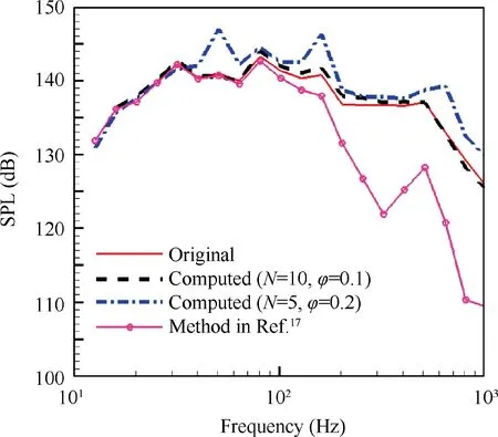
Fig. 8 Computational results with SAM.

As shown in Fig.8,the SAM can separate the background noise from the interested signal accurately in a broad frequency range. However, more sensor elements with a smaller loop gain will achieve remarkably higher computational precision. Compared with the SAM, the method introduced in Ref.17is influenced by the SNR. The higher the SNR, the weaker the coherence presented between the two kinds of sound sources and the better the results computed with the method in Ref.17. Fig. 8 shows that the SNR decreases remarkably when the sound frequencies exceed 100 Hz, thus a palpable error is generated when using the method in Ref.17to obtain the interested sound over 100 Hz.

As can be seen in Fig. 8, the upper limit of the interested frequency is 1 kHz. To extend the frequency range of interest,the half-length of a wave should be more than the minimum distance between any two sensors. Hence, the maximum frequency under investigation could be confined by the dimensions of the used sensors. The wave length corresponding to the maximum frequency should not be smaller than the diameters of the sensors.

4. Conclusions

Wall pressure fluctuations are mostly measured in a wind tunnel due to its reliability in simulating a turbulent boundary layer. However, the measurement results obtained by wind tunnel tests are usually contaminated by the background noise of wind tunnels.The jet and the valve noise are important contributors to the background noise in a transonic wind tunnel.In this study,a new method,the SAM,is developed to remove the background noise generated by the jet and the valve of wind tunnels.A salient merit of the SAM is that it can resolve the wall pressure fluctuations without knowing the exact information about the wall pressure fluctuations,such as the intensity, the decay factor, and the convection velocity.

The results of the investigation demonstrate that the SAM can separate the wall pressure fluctuations from the background noise accurately when they are at the same level. In addition, even when the wall pressure fluctuations are sometimes much lower than the background noise,the wall pressure fluctuations can still be picked up from the signals almost dominated by the background noise. The decay of wall pressure fluctuations changes the weighting of wall pressure fluctuations in the integrated signal of the background noise and the TBL noise. However, it does not affect the results of soundsource separation. Meanwhile, the sound-source separation based on the signal collected in a wind tunnel also reveals the effectiveness of the SAM for broad-band noise.

The precision of computation plays an important role in determining the wall pressure fluctuations separated from the background noise.Generally,the step length is inversely proportional to the precision of computation.Hence,two ways are suggested to increase the computational accuracy: (A) decreasing the loop gain or(B)increasing the sensors for signal collections.