Travel time prediction model of freewaybased on gradient boosting decision tree

Cheng Juan Chen Xianhua

(School of Transportation, Southeast University, Nanjing 211189, China)

Abstract：To investigate the travel time prediction method of the freeway, a model based on the gradient boosting decision tree (GBDT) is proposed. Eleven variables (namely, travel time in current period Ti, traffic flow in current period Qi, speed in current period Vi, density in current period Ki, the number of vehicles in current period Ni, occupancy in current period Ri, traffic state parameter in current period Xi, travel time in previous time period Ti-1, etc.) are selected to predict the travel time for 10 min ahead in the proposed model. Data obtained from VISSIM simulation is used to train and test the model. The results demonstrate that the prediction error of the GBDT model is smaller than those of the back propagation (BP) neural network model and the support vector machine (SVM) model. Travel time in current period Ti is the most important variable among all variables in the GBDT model. The GBDT model can produce more accurate prediction results and mine the hidden nonlinear relationships deeply between variables and the predicted travel time.

Key words：gradient boosting decision tree (GBDT); travel time prediction; freeway; traffic state parameter

Travel time is the most intuitionistic index to reflect the running condition, which is an important foundation for constructing intelligent transportation systems (ITS)[1]. With accurate travel time information, on the one hand, travelers can make better travel choices; on the other hand, traffic managers can improve traffic management decisions[2].

There are many methods for predicting the travel time, such as mathematical statistics methods[3-4]and machine learning methods[5]. Since the travel time prediction has typical nonlinear characteristics, the travel time prediction based on machine learning methods is more accurate than the methods based on mathematical statistics. Therefore, the travel time prediction method has gradually transferred to machine learning methods, such as artificial neural networks[6-7], support vector machines (SVM)[8-10], Kalman filters[11], the kernel-clustering algorithm[12]and theKnearest method[13-14]. A variety of models are proposed based on the methods. However, it is difficult for traffic researchers and managers to explain the relationship between indicators and the predicted travel time through these models. In view of this, the gradient boosting decision tree (GBDT) is used to build the travel time prediction model in this paper. GBDT combines the advantages of data mining to dig deep into the impact of variables on the predicted travel time.

The GBDT model provides a flexible framework to adopt different types of predictors as the input variables (for instance, traffic flow, speed, density, occupancy, number of vehicles, traffic state parameter and data-time variables). Meanwhile, the GBDT model understands the diverse influences of different variables on the predicted travel time, explores the nonlinear relationship between variables and the predicted travel time, and has good interpretability.

1 Travel Time Prediction Model Based on GBDT

GBDT is an iterative decision tree algorithm, which is based on the idea of boosting iteration. The foundation of GBDT is the classification and regression tree (CART) algorithm. Except for the first decision tree generated using the original indicator, the target in each iteration minimizes the loss function value of the current learner, that is, the loss function always falls along its gradient direction. By successive iterations, the final residual approaches zero. The results of all trees are added up as the final prediction result[15-17].

1) Initialize the learner, that is

(1)

wheref0(X) is the initial decision tree with only one root node;L(yi,c) is the loss function;yiis thei-th training data;cis a constant value that minimizes the loss function.

Travel time prediction is a regression problem. In GBDT, there are many loss functions for the regression problem, such as the squared loss function, absolute value loss function, and Huber loss function.The squared loss function used in the GBDT model is

(2)

wheref(x) is the learner obtained from the current iteration.

2) Let the number of iterations bem=1,2,…,M, and the negative gradient of thei-th training data is

(3)

According to all samples and their negative gradient direction (xi,gmi)(i=1,2,…,N), a decision treeTmconsisting ofJleaf nodes is obtained. Thej-th leaf node region isRmj(j=1,2,…,J). The best residual fitting value of each leaf is

(4)

The learner obtained in this iteration is

(5)

whereI(xi∈Rmj) is the explanatory function of thei-th training data in thej-th leaf node region, and

3) After them-th iteration, the final model is expressed as

(6)

Via the times that a variable appears in the decision tree and the performance of the model after each segmentation, the variable importance of the model can be obtained[17].

(7)

(8)

2 Data

In this paper, the VISSIM simulation software developed by PTV is used to analyze the travel time in the freeway. The length of 1 048.28 m between the airport interchange and Lukou interchange is selected as the research area.Time detectors are set at both ends of the selected freeway section. The route diagram is presented in Fig.1.

Fig.1 The study area

VISSIM simulation software is calibrated according to actual hourly traffic flow on the Nanjing Airport freeway from Nanjing to the Airport investigated at a airport toll station from 9:00 to 15:00 on August 22, 2017. Since the actual traffic flow does not include congestion, in order to cover the states of free-flow, transition and congestion in the freeway, the traffic flow is increased by 600 veh/h from the actual measured value of the previous period during 15:00—17:00, which reflects the congestion state. Only increasing the number of vehicles cannot lead to congestion. However, based on the state of transition, the authors guarantee that all variables are constant, and continue to increase the traffic flow to characterize the state of congestion.

Through investigation, the vehicle proportion of car, truck, bus and taxi on the freeway is 0.42∶0.12∶0.26∶0.2.

In the freeway, the expected speed distributions of car, truck, and bus is 120, 100, and 100 km/h. The speed distributions of cars, trucks, buses, and taxis are shown in Fig.2.

Using different random seed numbers, the experiment is simulated 133 times and the simulation time is 28 800 s. Finally, 133 sets of data are obtained, which represent 133 days’ data of 9:00—17:00. Data of 133 d are divided into two data sets, in which 27 to 133 d of data are used as training data sets and 1 to 26 d of data are used as test data sets.

The travel time is obtained at the sampling interval of 300 s.Tiis used to represent the travel time at time stepi(iis the current period), wherei=1,2,…,93, represents 93 time periods from 9:15 to 17:00 (The first three periods 9:00 to 9:15 are taken as the pretreatment time of VISSIM). Considering the short-term prediction of travel time,the prediction period is set to be 10 min ahead.

(a)

(c)

Fig.2Speed distribution. (a) Cars; (b) Trucks; (c) Buses; (d) Taxis

3 Establishment and Verification of the Model

3.1 Variables of the model

3.1.1 Traffic state parameter

In the Highway Capacity Manual[18], the freeway traffic state is divided into six grades (namely A to F) by means of average speed and density. As we all know, speed, density, and traffic flow are three basic parameters, which are interrelated. If the values of two parameters are known, the third one can be calculated. The standard of traffic state classification of a freeway is shown in Tab.1.

Tab.1 The standard of traffic state classification of a freeway[18]

In this study, traffic state parameters refer to the standard of traffic state classification of the freeway, letx=1,2,…,6 represent traffic states A to F, respectively. This paper combines existing traffic state levels and describes the freeway at a low level. Therefore, the traffic state of the freeway is divided into three categories.The free-flow state includes traffic states A and B, namely,xf=1,2. The transition state includes traffic states C and D, namelyxt=3,4. The congestion state includes traffic states E and F, namelyxc=5,6. The traffic state parameter isX={xf,xt,xc}.

The travel time is affected by traffic states. In order to clarify the impact of traffic states on travel time prediction, the traffic state parameter in current periodXiis introduced into the GBDT model.

3.1.2 Variables of the model

Traffic flow, speed, and density are three basic parameters that characterize traffic flow characteristics and affect the travel time of the vehicle. In addition, occupancy and the number of vehicles also have a certain impact on travel time. Therefore, traffic flow in current periodQi, speed in current periodVi, density in current periodKi, occupancy in current periodRiand the number of vehicles in current periodNiare introduced as input variables.

Other factors that have been discussed in previous studies[19]are also considered, that is,Tiis the travel time in current period;Ti-1is the travel time at time stepi-1;Ti-2is the travel time at time stepi-2; ΔTiis the change of travel time over two adjacent time steps, ΔTi=Ti-Ti-1; ΔTi-1is the changes of travel time over two adjacent time steps, ΔTi-1=Ti-1-Ti-2.

The target variable of the model, namely the predicted travel time, is the travel time at time stepi+1, which is denoted asTi+1.

3.2 Results and verification of the model

In GBDT, there are five parameters that need to be determined, namely, the number of leaf nodes in a single regression treeJ, learn rateη, the amount of attribute samplingSa, subsample fractionf, and the number of regression treesM. The paper uses data mining software Salford systems developed by the Salford Company of the United States to establish the GBDT model. After repeated experiments, all the parameters of the GBDT model are obtained, that is {J,η,Sa,f}={9,0.01,9,0.6}. The optimal number of regression trees based on the minimum value of the objective function is automatically determined. The number of regression trees is 923.

The training data sets are used to train the model, and the test data sets are used for testing. The results show that the error of the model in the training data sets is 3.59%, and that in the test data sets is 3.94%.

To test the effectiveness of the GBDT model, the back propagation (BP) neural network model with three-layer feedforward perceptron algorithm and the SVM model with radial basis function (RBF) as the kernel function are also established by using the same training data sets. Then, the same test data sets are used for testing.Tab.2 is the error of different models.

Tab.2 MAPE of different models %

3.3 Analysis of variables

The importance values of variables are determined in the GBDT model by the times of variables appearing in the decision tree. The relative importance value of the GBDT model is indicated in Fig.3. It can be seen from Fig.3 that the most important influence variable is the travel time in current periodTi. The travel time of the current period has the greatest influence on the travel time of the next period. As expected, the immediate previous traffic state will influence traffic in the near future. The influences ofRi, ΔTi,Ni, and ΔTi-1on the model are relatively small, indicating that the occupancy and the number of vehicles cannot directly affect the predicted travel time. The influence of the time difference on the model is less than that of the travel time of the two

Fig.3 The relative importance value

periods close to the predicted travel time.

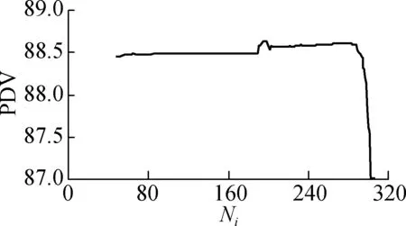
In the GBDT model, the partial dependency value (PDV) of the prediction model and each variable on the prediction results are shown in Fig.4. From Fig.4, each variable has a highly nonlinear relationship with the predicted travel time. TakingTias an example, whenTi<60 s, the PDV for the predicted travel time is the smallest fixed value, and the change ofTihas little effect on the predicted travel time. When 60 s180 s, the PDV for the predicted travel time becomes a fixed value again. The analysis results of the GBDT model show that the influences of the variableTiand the predicted travel time have a typical nonlinear relationship. Only when 60 s

3.4 Accuracy of the model

Fig.5 is a comparison between the travel time of the 5th day in the test data sets and the travel time obtained with different models. As indicated in Fig.5, the GBDT model can accurately predict the change of travel time.

4 Conclusions

1) The comparison of model prediction results shows that the error of the GBDT model is smaller than those of the BP neural network model and the SVM model.

2) In the GBDT model, travel time in current periodTihas the highest importance value. The travel time of the current period has the greatest influence on the travel time of the next period. As expected, the immediate previous traffic state will influence the traffic in the near future. The traffic state parameter in current periodXihas a greater influence on the predicted travel time, which is similar to the driving characteristics on the road. The number of vehicles in current periodNiand the time difference ΔTi-1have a small influence on the predicted travel time, indicating that the number of vehicles and the time difference cannot directly affect the travel time.

(a)

(d)

(g)

(j)

Fig.4The partial dependency value of each variable on the prediction result. (a)Ti; (b)Xi; (c)Ti-2; (d)Vi; (e)Ti-1; (f)Ki; (g)Qi; (h)Ri; (i) ΔTi; (j)Ni; (k) ΔTi-1

Fig.5 Error comparison of three models

3) The partial dependency value of the variable on the prediction results indicates that the GBDT model can accurately capture the nonlinear relationship between the variables and the predicted travel time.

4) The GBDT model will be applied to other research sections for verification in the subsequent study. However, data obtained by VISSIM limits diversity. In future research, the variables of weather, characters of drivers, and other variables (holidays, working days, non-working days, morning peak, evening peak and so on) affecting travel time will be considered in the GBDT model.