THE QUALITATIVE ANALYSIS OF A TWO SPECIES AMENSALISM MODEL WITH NON-MONOTONIC FUNCTIONAL RESPONSE AND ALLEE EFFECT ON SECOND SPECIES∗†

Xinyu Guan,Hang Deng

(College of Math.and Computer Science,Fuzhou University,Fuzhou 350116,Fujian,PR China)

Abstract In this paper,we present a two species amensalism model with non-monotonic functional response and Allee effect on second species.Local and global stability of the boundary and interior equilibrium are investigated.By introducing the Allee effect,we show that the boundary equilibrium have changed from unstable node and saddle into saddle-node.Also,the system subject to an Allee effect has increased the time of reach to its stable steady-state solution,but has no influence on the final density of the two species.Our results are supported by numeric simulations.

Keywords amensalism model;Allee effect;non-monotonic functional response;globalstability

1 Introduction

Amensalism is a basic interaction where a species inflicts harm to the other species without any costs or benefits received by the other.For example,the natural jump of locusts has severely reduced the quality of the caterpillar’s survival,see[1]and the references cited therein.

In 2003,Sun[2]proposed the following two populations amensalism model:where r1,r2,k1,k2and α are all positive constants.The author investigated the stability property of allthe possible equilibria of the system.

During the last decade,based on(1.1),many scholars[3-11]have investigated the dynamic behaviors of varies amensalism model and obtained many interesting results,which have greatly enriched and improved this direction.For example:For an amensalism system with strong generic delay kernel,the localasymptotic stability and the existence of Hopf bifurcation of the positive equilibrium were investigated in[4];sufficient conditions were obtained for the existence of positive periodic solution of a discrete amensalism model with Holling II functional response in[8];a two species amensalism model with a cover for the first species was investigated in[10],etc.

In particular,stimulated by the functional response of the predator-prey model,Wu[11]argued that it is necessary to use suitable functional response to discrete the relationship between the two species.Generally speaking,there is a saturating state between two species,so it is more practical to describe the saturation phenomenon using the non-monotonic type functional response[12,13].So the author proposed the following two species amensalism symbiosis model with non-monotonic functional response:

where a1,b1,c1,d1,a2,b2are all positive constants.The second species to the first one obey the non-monotonic functional response instead of linearize response.We notice that,adding this functional response in system(1.2)does not change any properties of the equilibrium,but only changes the stability conditions of the boundary equilibrium and the positive equilibrium.

It also brings to our attention that,to this day,still no scholars consider the influence of Allee effect to the amensalism model.Allee effect occurs when species depend upon predator saturation,evading natural enemies,cooperative predation or resource defense,selecting mates and increasing availability of mates[14-16],etc.At lower population densities,any of these factors can dominate.At this time,the Allee effect has great influence on the population.When the Allee effect is sufficiently strong,there is a critical threshold below which population behavior and dynamics may experience change.Consequently,the importance of the Allee effect has been widely recognized in many biological disciplines.

In recent years,there are many papers concerned with the Allee effects of the predator-prey system and competition system,see[17-24]and the references cit-ed therein.Stimulated by the works of[14,17,18],in this paper,we propose the following amensalism model with Allee effect on the second species:

(1)At lower population density,finding mate will be difficult,that is the individual searching efficiency β has decreased.Asβ→0 means that species rarely find a mate when the population density is less than a critical threshold.At this time→ 0 and the population is at risk of extinction.

(2)At a stable population density,searching mate efficiency of an individual will tend to be saturated.When the population is large enough,→ 1 means that for a population the effect of finding mate is almost nonexistent.

In order to calculate conveniently,we use the translation β=and system(1.3)becomes:

When system(1.4)is concerned,our aim is to determine the influence of Allee effect on system(1.4).We will present a qualitative analysis of equilibrium solutions of the model with Allee effect and compare the stability conditions with and without Allee effect.

We arrange the paper as follows:In the next section,we will investigate the local stability property of the equilibria of system(1.4).In Section 3,we will investigate the globalstability property of the boundary equilibrium and the positive equilibrium of system(1.4).In Section 4,two examples together with their numeric simulations are presented to show the feasibility of our main results.We end this paper by a brief discussion.

2 Local Stability

We now analyse the stability of steady-state solutions of system(1.4),which is subject to an Allee effect on the second population.The equilibria of system(1.4)is determined by the following equations:

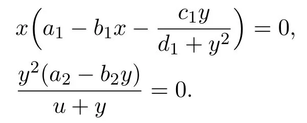
Obviously,system(1.4)admits four possible equilibria,E0(0,0),E1(,0),E2(0,)and E3(x∗,y∗),where

Obviously,E3is a positive equilibrium if and only if

Theorem 2.1E0(0,0)andare both saddle-nodes;is a saddle point ifholds and a stable node ifholds;the positive equilibrium E3(x∗,y∗)is a stable node if it exists.

ProofThe Jacobian matrix of system(1.4)at an equilibrium E(x,y)is

Now we have four cases to discuss the stability of equilibria of model(1.4).

Case 1For E0(0,0),we have

The characteristic equation of the variational matrix(2.2)is

Obviously,the two eigenvalues of J(E0)are λ1=a1>0 and λ2=0.Therefore,the equilibrium E0is non-hyperbolic and its stability is difficult to be judged directly from the characteristic root.In order to determinate its stability,we will use Theorem 7.1 in Chaper 2 in[25].

Firstly,using the translations X=−y,Y=a1x,d t=dτ,system(1.4)becomes:

Then expand system(2.3)in power series up to the fourth order around the origin and replace X,Y,τ with x,y,t for notational simplicity respectively.We get:

where P1(x,y)and Q1(x,y)are power series in(x,y)with terms xiyjsatisfying i+j≥5.Hence by Theorem 7.1 in Chapter 2 in[25],since the coefficient of x2is−<0,the equilibrium(0,0)of system(2.4)is a saddle-node.Consequently,E0of system(1.4)is also a saddle-node.That is,a neighborhood of E0is divided into two parts by two separatrices that tend to E0along the upside and the underneath of E0.The upper part is a parabolic sector,and the bottom part is consisted oftwo hyperbolic sectors(see Figures 1 and 3).

Case 2For E1(,0),we have

The characteristic equation of the variational matrix(2.5)is

Obviously,the two eigenvalues of J(E1)are λ1= −a1<0 and λ2=0.Just like equilibrium E0,the equilibrium E1is non-hyperbolic too.In order to determinate the stability of the equilibrium E1,we first transform the equilibrium E1to the origin by the translation(X,Y)=(x−,y),then expand the system in power series up to the fourth order around the origin,under which system(1.4)becomes:

where P2(X,Y)and Q2(X,Y)are power series in(X,Y)with terms XiYjsatisfying i+j≥5.

Then we let

be a matrix that transforms the Jacobian into a standard form.Under the transformation

where P3(x,y)and Q3(x,y)are power series in(x,y)with terms xiyjsatisfying i+j≥5.Similar to Case 1,since the coefficient of y2is−<0,the equilibrium(0,0)of system(2.9)is a saddle-node.Consequently,E1of system(1.4)is a saddlenode,and a neighborhood of E1is divided into two parts by two separatrices that tend to E1along the upside and the underneath of E1.One part is a parabolic sector,and the other is consisted of two hyperbolic sectors(see Figures 1 and 3).

Case 3For E2(0,),we have

The characteristic equation of the variational matrix is

The two eigenvalues of J(E2)are

where

The characteristic equation of the variational matrix is

Obviously,the two eigenvalues of J(x∗,y∗)are

One could easily see that to ensure the existence of the positive equilibrium,the assumptionis needed,in this case,λ1<0,λ2<0,which implies E3(x∗,y∗)is a stable node.The proof is completed.

3 Global Stability

Previously we have showed that under certain conditions the boundary equilibrium E2and positive equilibrium E3are both possible locally stable.An interesting issue is to find out the condition to ensure the global stability of those two equilibria.

To prove the global stability of the equilibria E2and E3,we need the following lemmas.

Lemma 3.1[26]Consider the following equation

Assume that function F(N)satisfies the following conditions:

(1)There is an N∗,such that F(N∗)=0.

(2)For all N∗>N>0,F(N)>0.

(3)For all N>N∗>0,F(N)<0.

Then N∗is globally stable.

Lemma 3.2The second species of system(1.4)is permanent.

ProofFrom the second equation of system(1.4),we set

Then

(1)There is a y∗=,such that F(y∗)=0.

(2)For all y∗>y>0,F(y)>0.

(3)For all y>y∗>0,F(y)<0.

Therefore,all the conditions of Lemma 3.1 are satisfied,and it follows from Lemma 3.1 that y∗is globally attractive.That is

Hence for all ε>0,there exists a T>0.For all t>T,we have

That is,the second species of system(1.4)is permanent.The proof is completed.

As a direct corollary of Lemma 2.2 of Chen[27],we have:

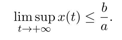
Lemma 3.3If a>0,b>0 and˙x≥x(b−ax),when t≥0 and x(0)>0,we have

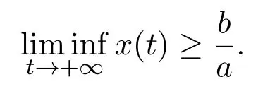
If a>0,b>0 and˙x≤x(b−ax),when t≥0 and x(0)>0,we have

Theorem 3.1Assume that,then the equilibrium E2(0,ab22)of system(1.4)is globally asymptotically stable.

ProofFrom the hypothesis,we have

which is equivalent to

Hence,for enough small ε>0,without loss of generality,we may assume ε<1 so that the following inequality holds

It then follows from Lemma 3.2 that for any ε>0,there exists a T>0,for all t>T,we have

From the first equation of system(1.4),(3.5)and(3.8),when t>T,we have

Hence,when t>T,we get

That is,

This ends the proof of Theorem 3.1.

Theorem 3.2The positive equilibrium E3(x∗,y∗)of system(1.4)is globally asymptotically stable if it exists.

ProofFirstly we prove that every solution of system(1.4)that starts inis uniformly bounded.From the first equation of system(1.4),we obtain

Thus,as a direct corollary of Lemma 3.3,one has

(3.13)together with(3.8)shows that there exist ε>0 and T>0 such that for all t>T,we have

And we consider the Dulac function g(x,y)=x−1y−2,then

By Dulac theorem,there is no closed orbit in area D.So E3(x∗,y∗)is globally asymptotically stable.The proof is completed.

4 Numeric Simulations

In this section,we will give two examples to validate the hypothesis of the main result.

Example 4.1Consider the following system:

Corresponding to system(1.4),we take a1=1,b1=2,c1=5,d1=1,a2=1 and b2=2.By calculation,we see that

(1)From Theorems 2.1 and 3.1,the equilibria E0(0,0)and E1(,0)are both saddle-nodes;the boundary equilibria E2(0,)is globally asymptotically stable(take u=1 and see Figure 1).

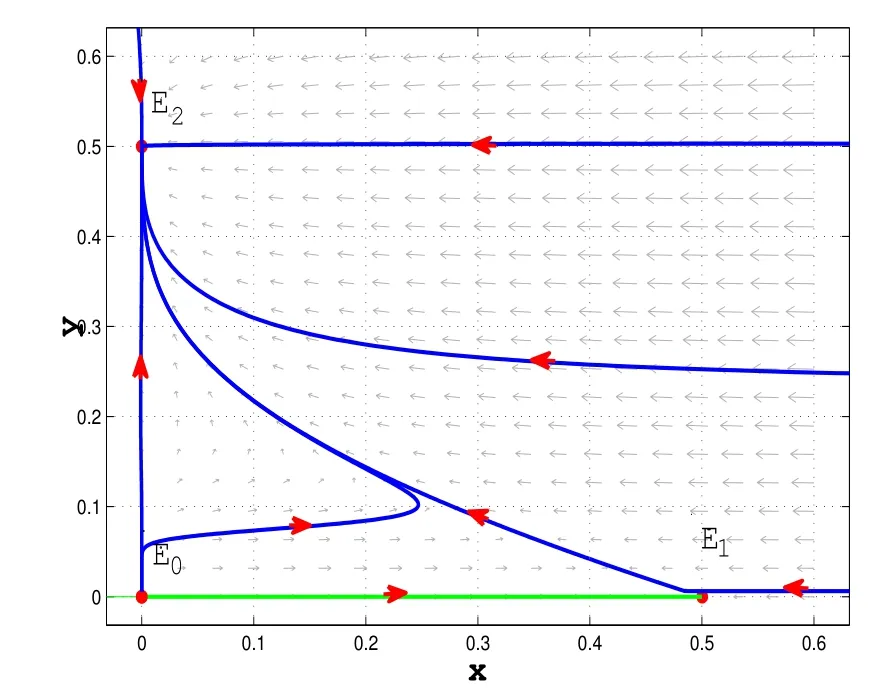
Figure 1:The phase portraits of system(4.1):E0 and E1 are saddle-nodes;E2 is globally asymptotically stable.

(2)The initial conditions are x(0)=1 and y(0)=2.The values of Allee constant u are respectively taken as 0,1,10.As u=0 means the system without Allee effect is considered(see Figure 2).

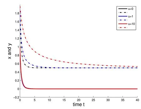
Figure 2:Time-population density graphs denoted by x(t)(solid line)and y(t)(dashed line)of system(4.1).

Example 4.2Consider the following system:

Corresponding to system(1.4),we take a1=1,b1=1,c1=1,d1=3,a2=1 and b2=1.By calculation,we see that

(1)From Theorems 2.1 and 3.1,the equilibria E0(0,0)and E1(1,0)are both saddle-nodes;the boundary equilibria E2(0,1)is a saddle;the positive equilibrium E3(,1)is globally asymptotically stable(take u=1 and see Figure 3).

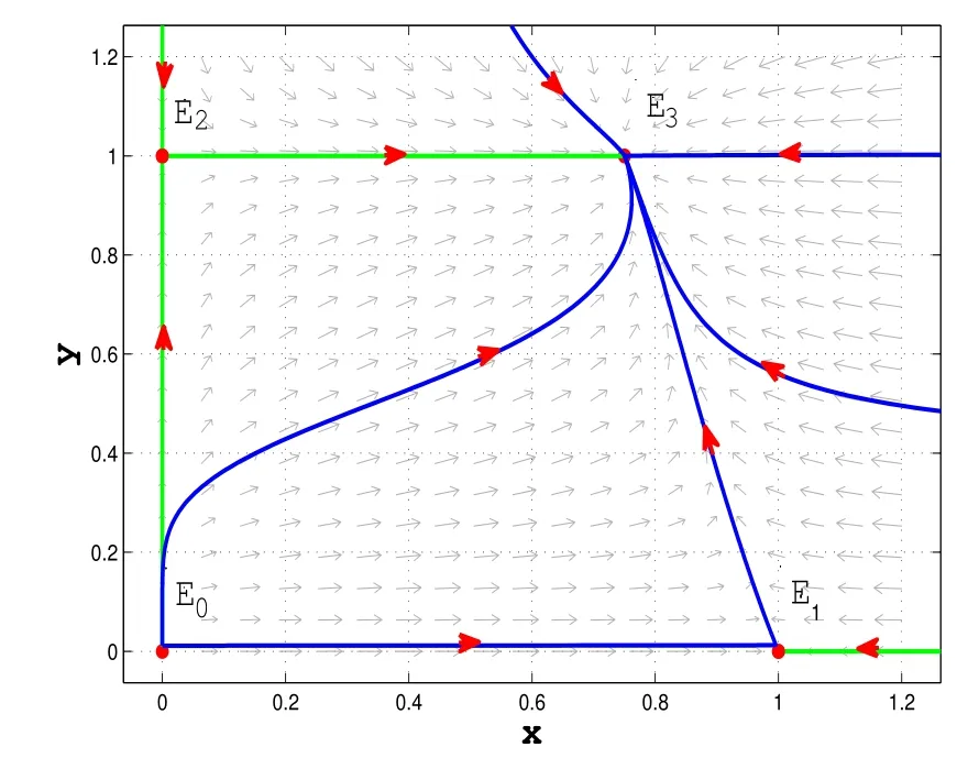
Figure 3:The phase portraits of system(4.2):E0 and E1 are saddle-nodes;E2 is a saddle and E3 is globally asymptotically stable.

(2)The initial conditions are x(0)=1 and y(0)=2.The values of Allee constant u are respectively taken as 0,1,10.As u=0 means the system without Allee effect is considered(see Figure 4).

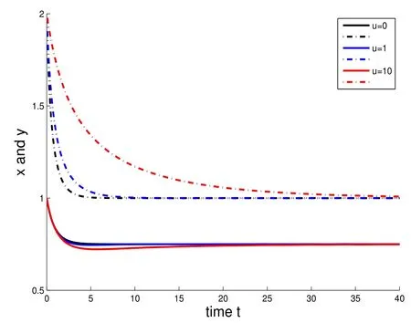
Figure 4:Time-population density graphs denoted by x(t)(solid line)and y(t)(dashed line)of system(4.2).

Figures 1 and 3 describe the properties of equilibrium points under different conditions.Figures 2 and 4 show that the trajectories of the system with and without Allee effect respectively.

5 Discussion

We propose a two species amensalism model with non-monotonic functional response and Allee effect on second species.As Huseyin Merdan[17]pointed out,Allee effects may have a stabilizing or a destabilizing effects on population dynamics.We find some interesting phenomenon when adding Allee effect:The boundary equilibria E1and E1change from unstable node and saddle to saddle node.The trajectories of the system subject to Allee effect approach the equilibrium solution more slowly than in the model without Allee effects and the bigger u is,the slower approaching to the equilibrium solution it is.But the Allee effect does not change the conditions of steady-state solutions.