THE CAUCHY PROBLEMS FOR DISSIPATIVE HYPERBOLIC MEAN CURVATURE FLOW∗†

Shixia Lv,Zenggui Wang

(School of Mathematical Sciences,Liaocheng University,Liaocheng 252059,Shandong,PR China)

Abstract In this paper,we investigate initial value problems for hyperbolic mean curvature flow with a dissipative term.By means of support functions of a convex curve,a hyperbolic Monge-Amp`ere equation is derived,and this equation could be reduced to the first order quasilinear systems in Riemann invariants.Using the theory of the local solutions of Cauchy problems for quasilinear hyperbolic systems,we discuss lower bounds on life-span of classical solutions to Cauchy problems for dissipative hyperbolic mean curvature flow.

Keywords dissipative hyperbolic mean curvature flow;hyperbolic Monge-Amp`ere equation;lifespan

1 Introduction

In this paper,we study the closed convex evolving plane curves under the dissipative hyperbolic mean curvature flow.More precisely,we consider such an initial value problem

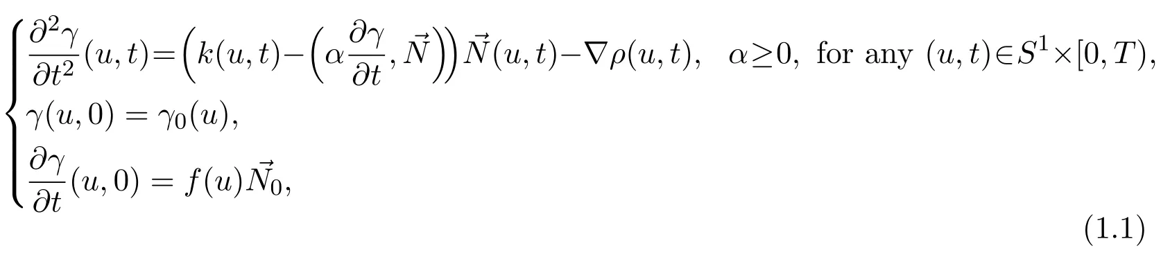
This system is an initial value problem for a system of partial differential equations for γ,which can be completely reduced to an initialvalue problem for a single partial differential equation for its support functions.The latter equation is a hyperbolic Monge-Amp`ere equation.Next we present a local existence theorem for the initial value problems(1.1).

Theorem 1.1(Local existence and uniqueness)Suppose that γ0is a smooth strictly convex closed curve.Then there exist a positive T and a family of strictly convex closed curves γ(·,t)with t ∈ [0,T)such that γ(·,t)satisfies(1.1),provided that f(u)is a smooth function on S1.

The following theorem has given the lifespan of classical solutions to the initial value problems.

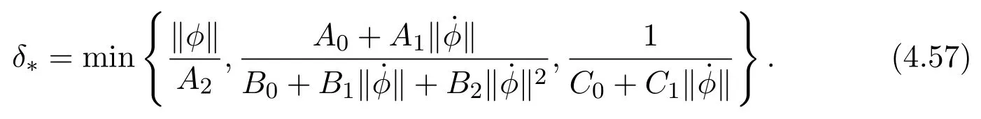
Theorem 1.2Suppose that γ0is a strictly convex closed curve,and f(u)is a smooth function on S1,then the lower bound δ∗of the local solutions of dissipative hyperbolic mean curvature flow is

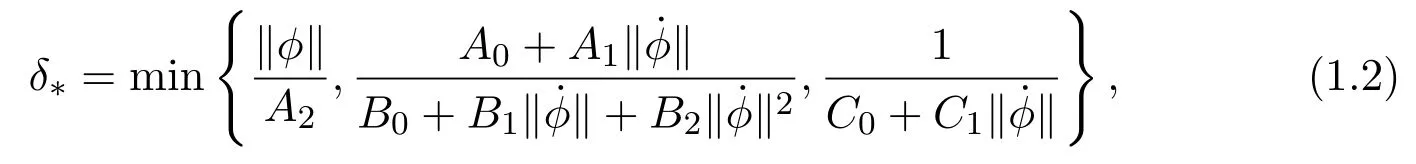
where,

It is well known that the elliptic and parabolic partial differential equations have been successfully applied to differential geometry and physics,such as Hamilton’s Ricci flow and Schoen-Yau’s solution to the positive mass conjecture[1,2].It is na-tural and important to apply the well-developed theory of hyperbolic differential equations to solve problems in differential geometry and theoretical physics.Motivated by the work of Ricci flow,Kong,Liu and Dai introduced and studied the hyperbolic geometric flow[3-7].

The study of hyperbolic mean curvature flow(HMCF for short)can be dated back to Gurtin and Podio-Guidugli[8],where they developed a hyperbolic theory for the evolution of plane curves.Rostein,Brandon and Novick-Cohen[9]studied a hyperbolic theory by the mean curvature flow equation

where vt,β,v and k are the normal acceleration of the interface,dissipation coefficient,normal velocity and mean curvature of the curve,respectively.In[9],a crystalline algorithm was developed for the motion of closed polygonal curves.Yau[10]proposed and studied the motion of a hypersurface whose acceleration is equalto its mean curvature along the normal direction.He,Kong and Liu[11]investigated this problem and gave the short-time existence theorem.However,it can not be reduced to a Euclidean invariant hyperbolic equation.Lefloch and Smoczyk[12]established a hyperbolic normal mean curvature flow:

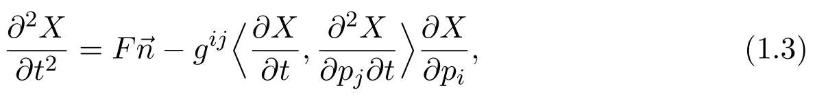
where F is the driving force and gijis the inverse of the induced metric on the hypersurface X(p,t)in Rn+1.In the case of,this normalflow can be derived from a Hamiltonian principle,and it possesses some conservation laws.To proceed,the hyperbolic shortening problems,that is,taking F as the curvature of a plane curve and n=1,are studied in Kong,Liu and Wang[13],and they proved the formation of singularities in finite time and asymptotic behavior of the flow under certain conditions.Furthermore,[13]studied the following flow

and illustrated the close relationship between the HMCF and the equations for evolving relativistic strings in the Minkowski space R1,1.In Kong and Wang[14],several criteria on finite time blow-up for graphs were obtained,where they proved that the singularities must develop in finite time if the total variation of initial curve is small enough in one period under some certain conditions and the lifespan was also given.

Recently,Li and Wang[15]investigated the life-span of classical solutions to Cauchy problems for one-dimensional HMCF[12].He,Huang and Xing[16]studied the self-similar solutions to the hyperbolic mean curvature flow for plane curves.More precisely,they considered the following immersed plane curve:

Here,F0:R→C is the immersed initialcurve and it is assumed to be nonzero.f,g:I→R and H:I→C are differentiable with f(0)=0,g(0)=1 and H(0)=0.[16]proved that all self-similar solutions evolved under the hyperbolic mean curvature flow are either straight lines or circles.Ginder and Svadlenka[17]proposed the numerical simulation for plane curves under dissipative hyperbolic mean curvature flow.Mao[18]studied forced hyperbolic mean curvature flow,proved the local existence uniqueness and generalized the corresponding results in[11]and[13].

Compared with the studies of hyperbolic mean curvature flow in[11-14],a new kind of more physical hyperbolic mean curvature flow was established by Notz[19],where the motivation of this flow was closed hypersurfaces moving that driven by mean curvature and inner pressure.Meanwhile,the local existence of smooth solutions and the stability with respect to the initial data were obtained.After that,Yan[20]studied the large time existence for the motion of closed hypersurfaces in radially symmetric potential and introduced a quasi-linear degenerate hyperbolic equation which describes the motion of the surfaces extrinsically.Chou and Wo[21]proposed a hyperbolic Gauss curvature flow for convex hypersurfaces,and the graph of the hypersurface under this flow gives rise to a new class of fully nonlinear Euclidean invariant hyperbolic equations.Particularly,Wo,Ma and Qu[22]introduced a new hyperbolic version of affine invariant curve flow,obtained the localsolvability and finite time blow-up,and discussed some group-invariant solutions to this flow.Recently,Wang[23]proved the lifespan of classical solutions to Cauchy problems for hyperbolic mean curvature flow with a linear forced term.In[24],the evolution of plane curves under HMCF with different constant externalforced term was studied.Furthermore,Wang[25]investigated symmetry reduction and group-invariant solutions to hyperbolic mean curvature flow with a constant forcing term.Wang[26]introduced a new hyperbolic mean curvature flow in Minkowski space R1,1,and proved singularities formation of spacelike curves under hyperbolic mean curvature flow.Subsequently,Wang[27]proposed a new hyperbolic affine geometric flow,and generalized the corresponding results in[22].However,to our knowledge,the dissipative hyperbolic mean curvature flow has not been studied yet.

Noting the dissipative property of(1.1),we expect that the dissipative hyperbolic geometric flow admits a global smooth solution for all t≥0.In this paper we focus on the initial values problems for the dissipative hyperbolic mean curvature flow.In the future,we will study the global existence of the solutions to the dissipative hyperbolic mean curvature flow.Furthermore,for a closed curve,we will give the behavior of the plane curve under the dissipative hyperbolic mean curvature flow.

The paper is organized as follows.In Section 2,we derive a hyperbolic Monge-Ampre equation by the dissipative hyperbolic mean curvature flow and give the short-time existence theorem.In Section 3,we reduce the hyperbolic Monge-Amp`ere equation to quasilinear hyperbolic systems in terms of Riemann invariants and get the localexistence ofthe flow(1.1).In Section 4,we prove the main result using the local solutions theory for Cauchy problems with respect to quasilinear hyperbolic system.

2 Hyperbolic Monge-Amp`ere Equation

In the study of the motion of convex curves,it is useful to express the flow in the terms of the support functions rather than the graph.Let us denote θ to be the unit outer normal angle for a convex closed curve γ:S1→R2.Hence,

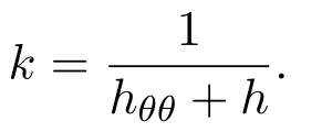
based on Frenet formula,then we have=k.

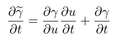
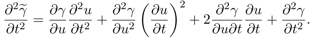
Suppose thatγ(u,t):S1×[0,T)→R2is a family of convex curves satisfying the dissipative hyperbolic mean curvature flow(1.1).Let us use the normal angle to parameterize each convex curve γ(·,t),that is,set

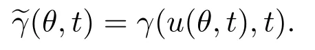
Use the chain rule,

and

The support functions of γ are given by

Then,we have

Hence,the curve can be represented by the support functions

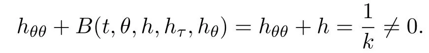
Thus all geometric quantities of the curve can be represented by the support functions.In particular,by the definition of the support functions,the curvature can be written as

We know that the support function h(θ,t)satisfies

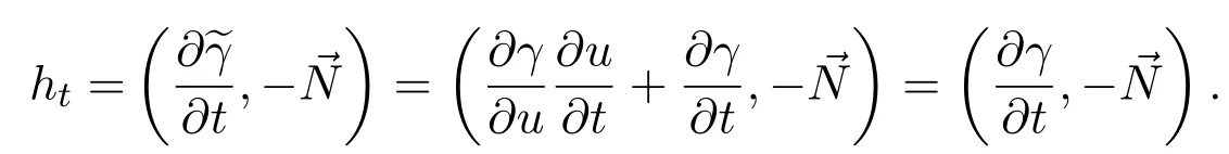
Moreover,

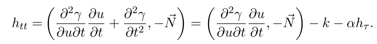
In terms of the normal evolving curve,we have

Using the formula

we get

Hence,the support function h(θ,t)satisfies

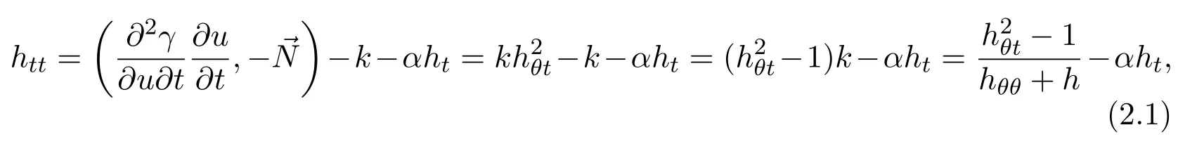
namely,

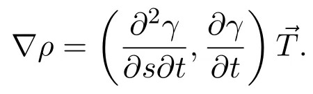
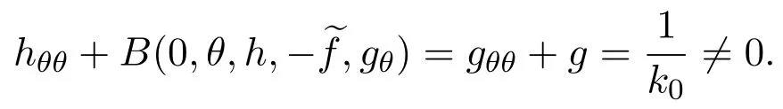
Then,it follows from(1.1)that

where g is the support function of γ0,andis the initial velocity of the initial curve γ0.

For an unknown function z=z(θ,t)defined for(θ,t) ∈ R2,the corresponding Monge-Amp`ere equation reads

the coefficients A,B,C,D and E depends on τ,θ,z,zt,zθ.We say that the equation(2.4)is a hyperbolic Monge-Amp`ere equation,if

and

It is easy to see that equation(2.2)is a hyperbolic Monge-Ampre equation,in which

In fact,

and

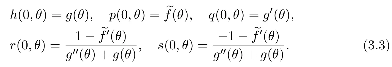
Furthermore,if we assume that g(θ)and(θ)are third and twice continuous by differentiable on the real axis respectively,then the initial conditions satisfies

and

It then follows directly from the standard theory of hyperbolic equations[28]that Theorem 1.1,that is the local existence and uniqueness theorem is proved.

3 Equations for Riemann Invariants

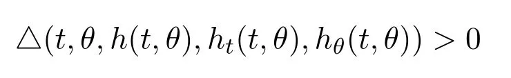
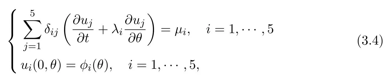
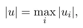
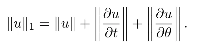
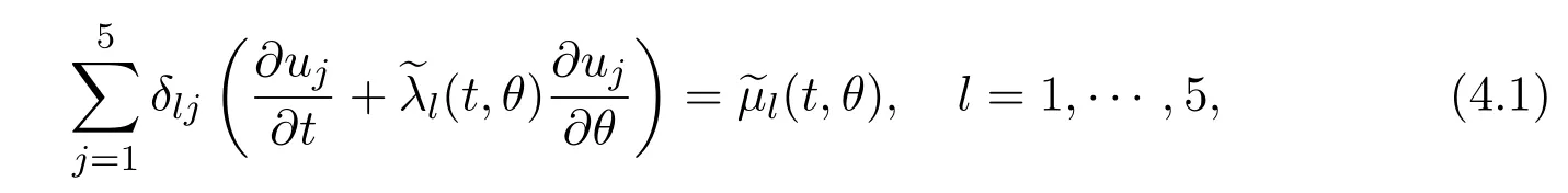
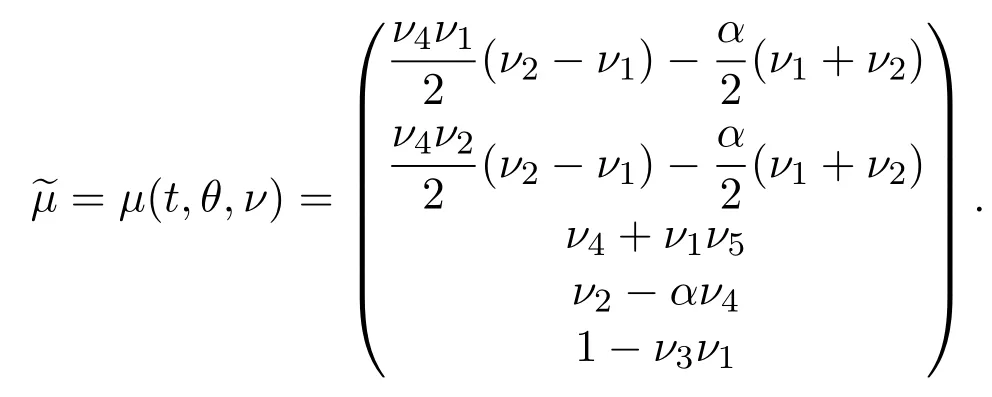
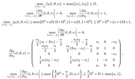
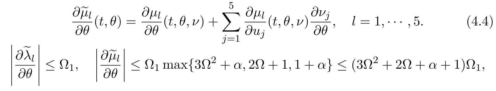
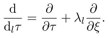
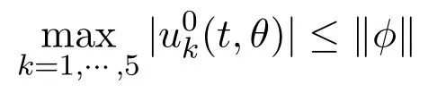
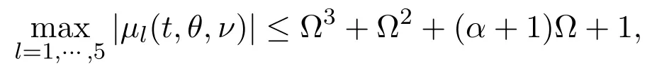
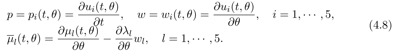
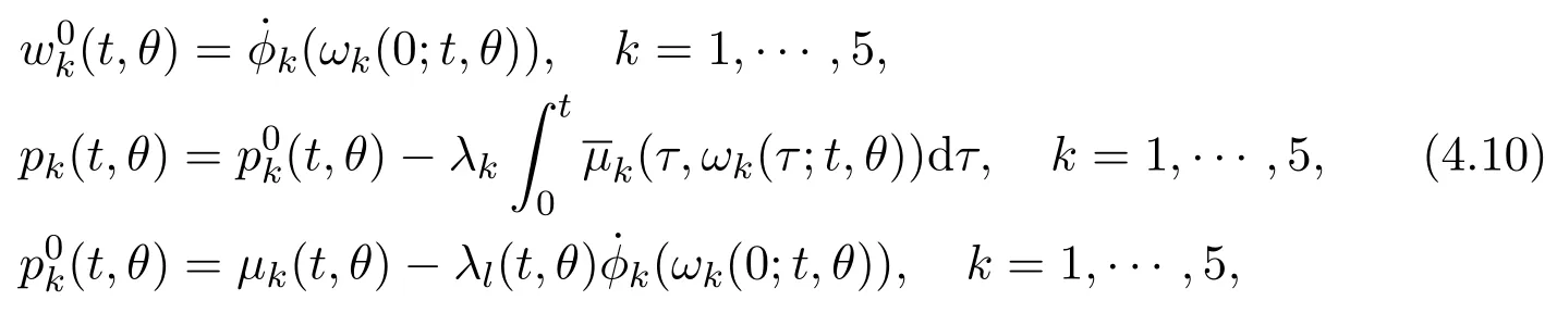
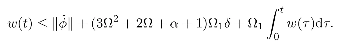
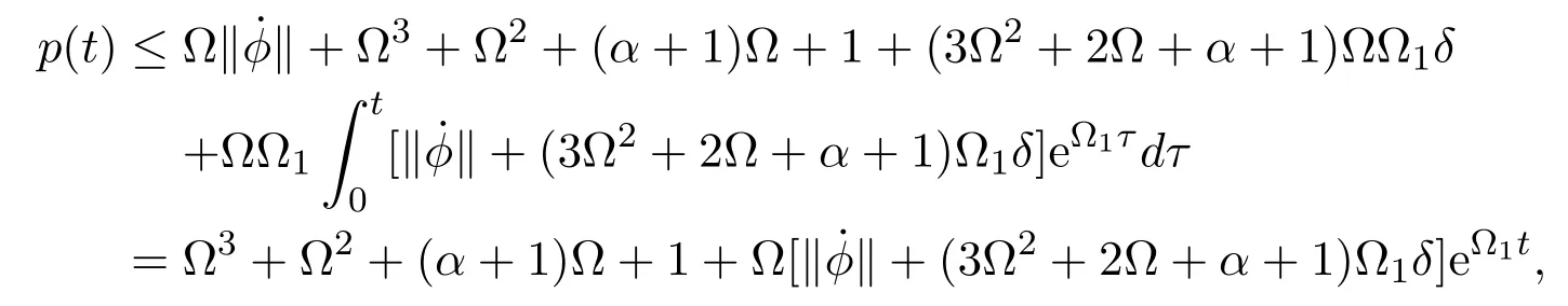
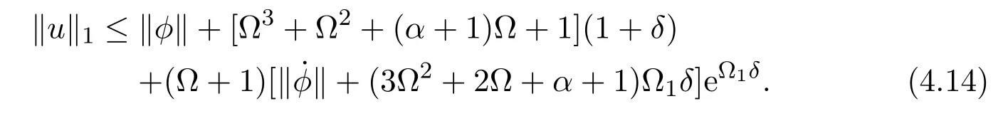
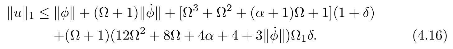
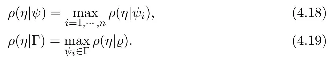
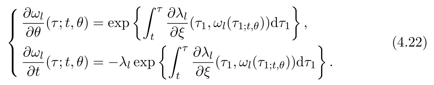
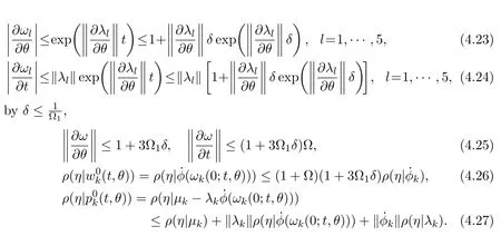
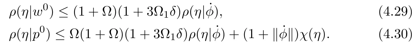
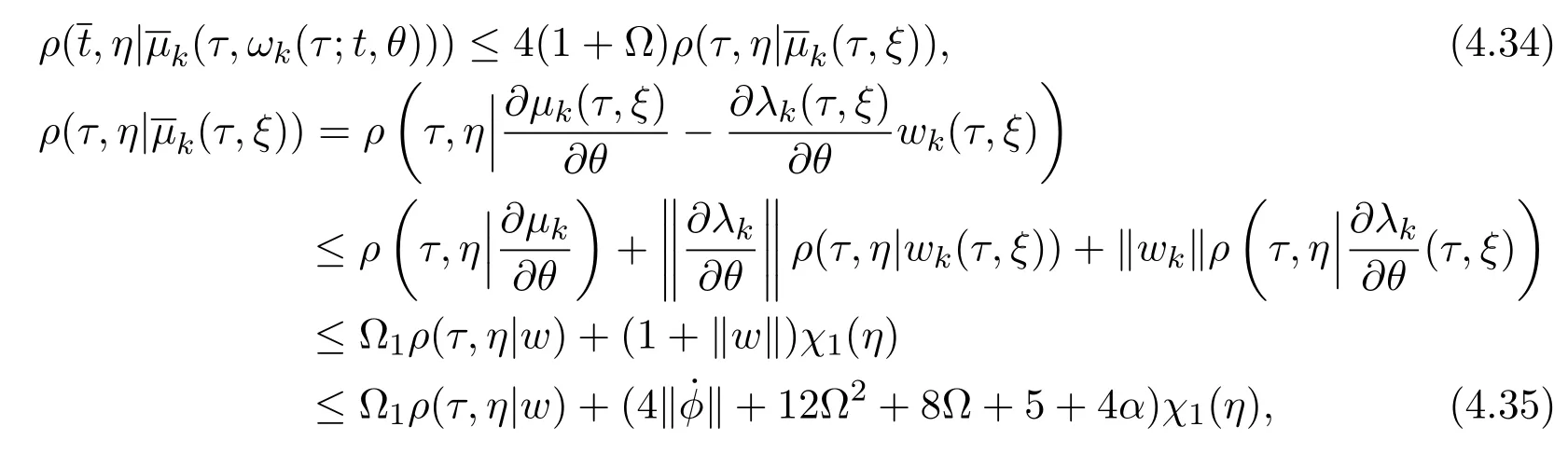
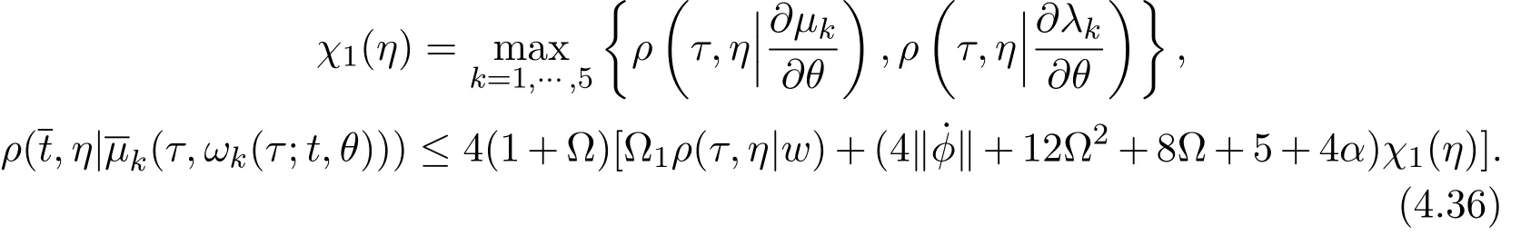
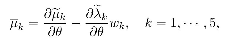
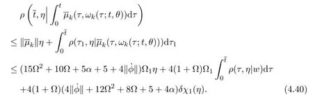
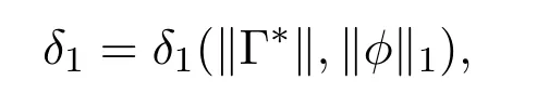
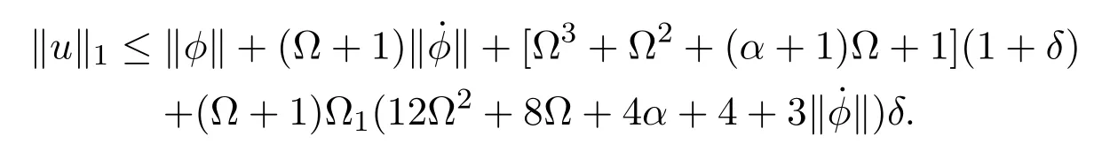
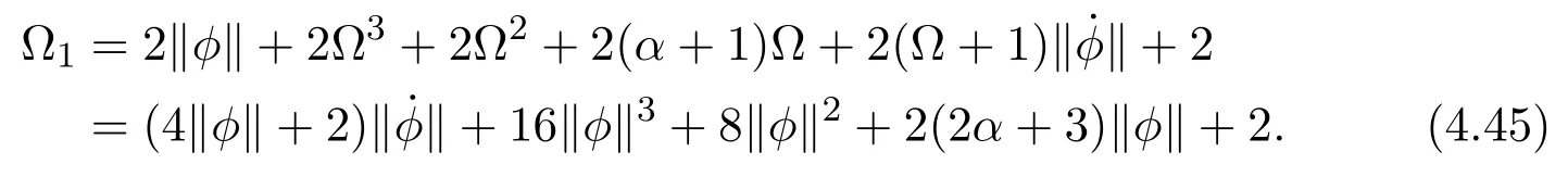
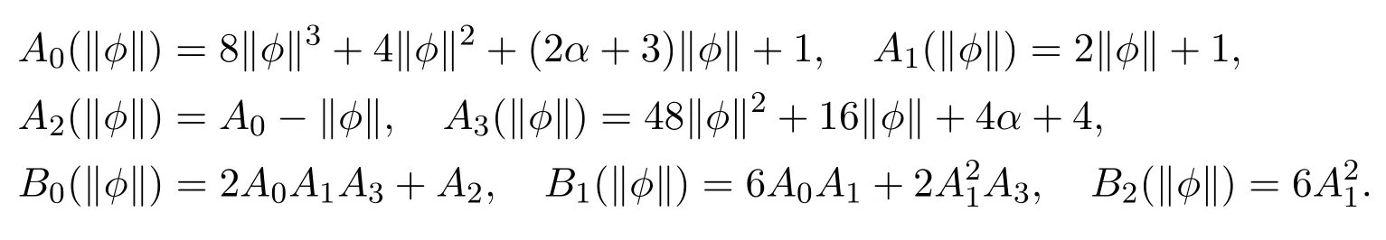
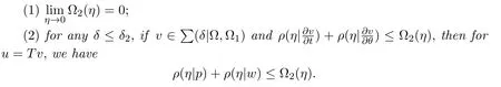
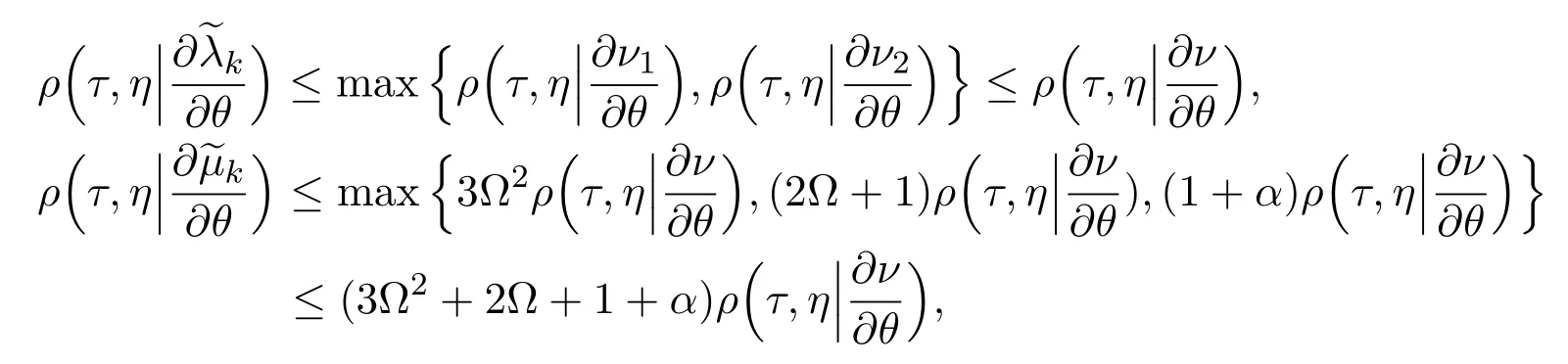
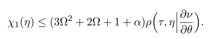
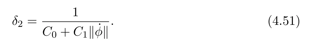
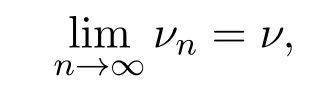
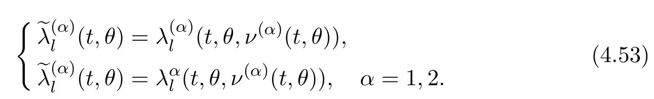
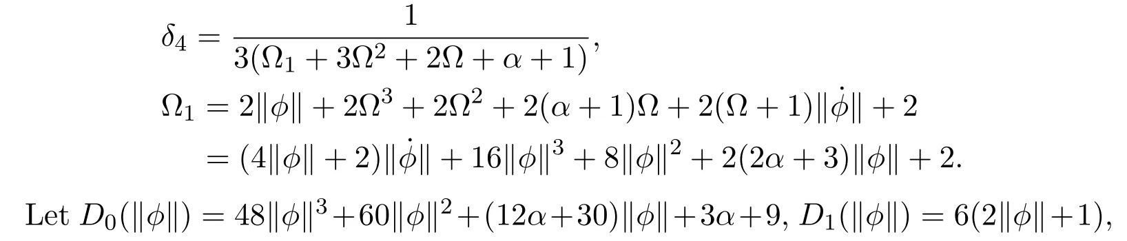
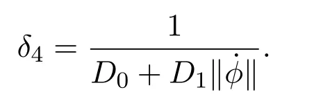
This section is concerned with the reduction of(2.2).Let h(θ,t)be a C3-solution of equation(2.2)in some domain={(θ,t)|0 ≤ θ≤ 2π,0

The inequality means that vertical lines t=const.are free.By definition,put

The functions r and s are tangents of angles of inclinations of characteristics of equation(2.2),we always call them Riemann invariants of(2.2).Let p=ht,q=hθ,then

Theorem 3.1Let h(θ,t)be a C3-solution of(2.3).Suppose(3.1)and(2.3)are satisfied by h.Then the set of functions(r,s,h,p,q)(where r,s we get from(3.1),p=ht,q=hθ)is a C1-solution of the systems of five equations(3.2)in.

Theorem 3.2Let(r,s,h,p,q)be a C1-solution of(3.2)in the domain.Let initial values for this solution be

holds.Then h(θ,t)is a C3-solution of(2.3)in the domain e D,furthermore,ht=p,hθ=q,hθθ+h0 hold.

If let u=(u1,u2,u3,u4,u5)T=(r,s,h,p,q)T,

Then we reduce equation(3.2)to Cauchy problems of quasilinear hyperbolic systems in Riemann invariants.

in which,

Firstly,suppose ϕ =(ϕ1,···,ϕ5)Tis bounded on e D and ϕ ∈ C1(e D).Take a suitable positive constant Ω,such that

where model∥ ·∥ is on the C0space.Throughout this paper,we use the following notation:The absolute value of any vector u=(ui)is defined as

and the C0norm of a vector function u=u(t,θ)=(ui(t,θ))on a domain R is defined as

For the continuous differentiable vector function u(t,θ),we may define

Furthermore,for any finite function setΓ,we can similarly define its norm ∥Γ∥,∥Γ∥1.

Denote R(δ0)={(t,θ)|t∈ [0,δ0],θ ∈ R},and define it’s exterior domain E(δ0)={(t,θ,u)|(t,θ) ∈ R(δ0),|u|≤ Ω}.Furthermore,supposeare C0functions defined on E(δ0),then by the standard hyperbolic theory[29],there exists a constant 0< δ∗≤ δ0,such that Cauchy problems of(3.4)has a unique C1solution u(t,θ)on R(δ∗).

4 The Proof of Theorem 1.2

In this section,we consider the life span of the solutions by the construct method of the local solutions for Cauchy problems of quasilinear hyperbolic systems in[29].

Next we give the proof of Theorem 1.2.

Firstly,we consider quasilinear hyperbolic systems(3.4)to be linear.Take a suitable positive constant Ω1,such that

Here Ω1is a positive constant derived from the second priori estimate.Define the following functions set

For any ν ∈ Σ(δ|Ω,Ω1),by the linear hyperbolic systems,

and the initial conditions ul(0,θ)= ϕl(θ),θ∈ R1,l=1,···,5,in which(t,θ)=λl(t,θ,ν),that is,=(ν2,ν1,ν1,ν2,ν1)T,(t,θ)=µl(t,θ,ν),that is,

Hence,C0norm of theΓ∗is

Let

then we have

hence,C0norm of the set Γ2[ν]is

Next,we will get some priori estimates for the solutions of Cauchy problems for linear hyperbolic systems.These estimates will be useful in proving the existence and uniqueness of solutions for initial value problems of quasilinear hyperbolic systems.

Firstly,using the first associated integral relations of the initial value problems(4.4),we obtain

By

and

if 0≤ t≤ δ,we have

This is the first priori estimate for the solutions of Cauchy problems.

We are going to construct the second priori estimate for the first derivatives of the solutions to Cauchy problems.Denote

Based on the second associated integral,

and

on R(δ),we have

Let

obviously,we have

By integral relations,if 0≤ t≤ δ,

Based on Gronwall inequality,

we have

Using(4.11),we have

that is,

By the definition of∥u∥1= ∥u∥+∥p∥+ ∥w∥,

Without loss generality,we assume δ0≤and restrict to δ∈ (0,δ0),then

Based on Taylors expansion,

Plug(4.15)into(4.14),and simplify the second order term of δ,then there is

This is the second priori estimate for the first derivatives of the solution of the Cauchy problems.

Next,we are going to estimate the modulus of continuity of the first order derivatives of the solution.Let ψ(t,θ)be a function on the bounded domain R.The modulus of continuity of ψ(t,θ)are defined by the following non-negative function:

Similarly,we can define the modulus of continuity of a function with any number of independent variables.Moreover,the modules of continuity of a vector function ψ = ψi(t,θ)(i=1,···,n)or a set of functions Γ = ϱ can be defined as follows:

Using an ordinary equation where θl= ωl(τ;t,θ)satisfies

and the initial conditions

It is easy to see that,

Hence,

Denote χ(η)=max{ρ(η|µk),ρ(η|λk)},then

Hence,we have

Furthermore,

Define

By the second integral relations(4.9)and(4.11),we will estimate ρ(τ,η|w)and ρ(τ,η|p)for≤ δto get

in which,

By

we have

that is,

By the properties of the continuity modulus,

we have

Hence

using Gronwall inequality and t≤ δ< δ0<,we have

By Cauchy problems of the linear hyperbolic systems,there exists a unique continuous differential solution u=(ui(t,θ)).Denote u=T v.Obviously,a fixed point of the operator T is a solution of the initial value problems.Therefore,it is sufficient to prove that the operator T has a unique fixed point,provided that δ>0 is suitably small.We first prove that there exists a positive number δ1≤ δ0depending only on the norm ∥Γ∗∥ and ∥ϕ∥1:

such that for any δ≤ δ1,the operator T maps ∑(δ|Ω,Ω1)to itself.To do so,we use the first priori estimate(4.7)and the second priori estimate(4.18)to bound ∥u∥and ∥u∥1.It follows that for u=T v,we have on R(δ)that

Taking Ω =2∥ϕ∥,we have

then∥u∥≤ Ω,

Take

Let

Then we can choose

Take

If δ≤ δ1,the operator T maps Σ(δ|Ω,Ω1)to itself.

Now we will use the third priori estimate(4.42)to prove the following lemma.

Lemma 4.1There exists a positive numberand a nonnegative function Ω2(η)(0< η< ∞),such that

ProofLet.By the definition of the modulus of continuity and the construction ofΩ1,we have(4.42)and

where

By

we have

Denote

then we take

Let

then

Then if 0< δ< δ2,Lemma 4.1(1)-(2)hold.The proof is completed.

Take δ3=min{δ1,δ2},and introduce functions set

then the operator T maps Σ(δ3)to itself.It is easy to see that T is compact on C1[R(δ)]and closed with respect to the C0norm.We now prove that there exists a positive numbersuch that the operator T is a contraction operator with respect to the C0norm on R(δ∗).

Firstly,under the C1norm,the set Σ(δ3)is bounded and equicontinuous,hence it is precompact.Assume

then

Hence the set is compact in C1[R(δ)].Moreover Σ(δ3)is closed with respect to the C0norm(because ∥ν∥ ≤ ∥ν∥1,the convergence under the C1norm provides the convergence under C0norm,hence it is complete with respect to C0norm).Hence we only need to prove that there exists a δ∗≤ δ3,such that the operator T is a contraction operator in R(δ∗).If we can show this,the existence of a unique fixed point for T will be proved.

Let ν(1),ν(2)∈ Σ(δ3),then u(1)=Tν(1),u(2)=Tν(2)∈ Σ(δ3).Assume ν∗=ν(1)−ν(2),u∗=u(1)−u(2),and

Then we have

where

Now notice that on R(δ),we have

By the first estimate,we have

Take

then we have

If we choose δ∗=min{δ3,δ4},the operator T is a contraction operator on R(δ∗).

From the above,by

we get δ2< δ4.Hence,the lower bound of the local solutions of Cauchy problems δ∗is

The proof of Theorem 1.2 is finished.

Remark 4.1If α=0,we can get the lower bound of the existence interval of the solutions.The solutions are obtained from the Cauchy problems of hyperbolic mean curvature flow without dissipative term.If α0,δ∗becomes smaller and smaller as α becomes larger and larger,hence,the dissipative coefficient δ∗has an effect on the existence of the solutions.

Remark 4.2By the expression of δ∗,for any initial conditions we cannot get δ∗→∞.This shows that no matier what the initial value is,C1solution cannot be ensure to exist in larger area.Because there is a constant term 1 in the last equation of quasilinear hyperbolic systems in terms of Riemann invariants.

Remark 4.3[15]studied the normal hyperbolic mean curvature flow.In this paper,we have successfully applied its methods to discuss the dissipative hyperbolic mean curvature flow.

Acknowledgements The author is very grateful to the referees for their comments and suggestions which have led to a significant improvement of the paper.