Best practices for model-based and simulation-aided engineering of power transmission and motion control systems

Jean-Charles MARE

Institut Clément Ader(CNRS UMR 5312),INSA-Toulouse,Toulouse 31077,France

KEYWORDS Actuator;Aerospace;Architecture;Causality;Modelling;Motion control;Power transmission;Simulation

Abstract This paper deals with the modelling and simulation of aircraft systems,in particular for power transmission and control.It is intended to review,propose and disseminate best practices for making model-based/simulation-aided engineering more efficient at any phase of the system life cycle.The proposals are aimed at creating value,not only by increasing the performance of the product under study but also by shortening the time to market,capitalizing knowledge,mitigating risks and facilitating concurrent engineering.The needs associated with the engineering activities are firstly identified to define a set of requirements for the models.Then,these requirements are used to drive the considerations leading to model development,focusing in particular on the process,modelled physical effects,modelling level,model architecting and concurrent engineering.The third part deals with the model implementation,giving special consideration to the different types of models,causalities,parameterization,implementation and verification.Each part is illustrated by examples related to safety critical actuators.

1.Introduction

Modelling and simulation are being used more extensively every day in systems engineering at any step of the life of a product.On the one hand,the offer of commercial numerical simulation environments has become huge and broad.On the other hand,better scientific understanding and modelling of physical effects combined with continuous progress in computer science are pushing back the limits of simulation fidelity and rapidity.Today’s modelling and simulation(M&S)potentially offers a tremendous means to increase performance at reduced risk while saving time and money.Decision making is enhanced through rapid assessment and early validation of specifications,architectural choices,sizing,integration,operation,maintenance,training,troubleshooting,and even deconstruction.

The use of Finite Element Modelling(FEM)has been well established since the 1970s for stress and strain analysis in solid mechanics.The use of given commercial software is even accepted for aircraft certification by the regulatory authorities,e.g.the Federal Aviation Administration(FAA).The status is far different for system-level simulation,which started to expand commercially 20 years later.This delay mainly comes from the multiple aspects to be dealt with:

-Multiphysics.Especially for mechatronic systems like flight controls,landing gears,and engine control,which involve solid and fluid mechanics,electromagnetism,electricity,electronics,heat transfer,etc.

-Multiscale.Lumped or distributed effects,e.g.in flight controls(2 lumped forces on the control surface on which distributed aerodynamic forces act),and slow or fast dynamics(e.g.power electronics switching time in actuators and actuator thermal time constant in a ratio of 1:1000).

-Multilevel.Whole system,system,subsystem,equipment,component,part(e.g.air transportation,aircraft, flight controls,actuator,servovalve,spool valve).

-Multi-activity. Architecting, sizing, control synthesis,response to faults,thermal balance,peak power demand,etc.

-Aircraft,like any embedded system,impose very antagonistic considerations(e.g.energy consumption,weight and envelope,reliability and autonomy,environment friendliness)that make compromises hard to find.Some general documents paving the way towards the standardization of the development and simulation of system level models have already been published.However,these are quite recent documents that are either dedicated to a specific phase of M&S or to a specific field of application,or are reserved for a company’s internal use:

-The IEEE(Institute of Electrical and Electronics Engineers)standard 1516,1first published in 2000,is a capstone document of a series of standards issued by the IEEE computer society.They describe a unified approach for the construction of interoperable simulation systems.M&S is viewed essentially at computer and information systems levels.

-The NASA(National Aeronautics and Space Administration)technical standard NASA-STD-7009A,2first issued in 2008,was initiated after the investigation of the loss of Space-Shuttle mission STS-107.3It focuses on engineering and technical requirements for models and simulation developed and used in NASA programmes.It includes 39 requirements and 48 recommendations that serve 7 main objectives covering the whole life cycle of a model.

-The FMI(Functional Mock-up Interface)standard,4first issued in 2010,was developed by 16 companies and research institutes under the aegis of the Modelica Association.It aims to standardize the interface between dynamic simulation environments so that tools can be coupled through exchange of models or co-simulation.

-The aerospace information report AIR6326,5first issued in 2015,focuses on definitions,in particular for modelling levels.It establishes basic terms and definitions applicable for modelling and simulation of aircraft electric power systems.A substantial part of the document is dedicated to the illustrative example of the electric power system of a more electric aircraft.

-Airbus Procedure AP2633,6initiated the late 1990s,is an example of a document developed in the context of a given enterprise.It focuses on a general description relative to the model for exchange between partners(roles and responsibilities,process and model description).7

Unfortunately,there is still a lack of shared and commonly applied best practices in M&S,in particular in the field of power transmission and motion control systems.This deprives engineers of the possibility of taking best advantage of M&S in mixed collaborative and competitive industrial contexts.The simulation tools are available and efficient(e.g.Matlab-Simulink©,AMESim©,Saber©,Dymola©)but,at system level,there is still a need to develop and standardize best practices to fully exploit the opportunities offered by commercial system-level simulation environments.

According to the author’s experience after more than 30 years of activity in M&S in academia and industry,three major considerations have to be kept in mind for efficient creation of value through simulation:

-M&S should not be seen as an objective in itself.Instead,it should be perceived as an enabling activity to support understanding and decision making.

-The model should be considered as a product in itself,with all its phases of life,including needs and requirements,architecting, integration, verification and validation,deployment(documentation,training and support),and upgrades.

-There is no universal model that can be used in all circum

stances,like a ‘‘Swiss army knife”.Instead,a model has to be developed to meet given engineering needs for a given domain of operation.

These important points of view have driven the following developments in the particular case of embedded power systems(although most of the proposal can be extended to other applications).The main intention is to better meet project needs and to progress towards increased acceptance of system-level M&S by the regulatory agencies and authorities.Section 1 is dedicated to the model requirements.Section 2 deals with the model development.Section 3 focusses on its implementation.An appendix summarizes the most important definitions regarding modelling and simulation.

2.Requirements based modelling and simulation

2.1.Global needs

Most of the time,the very first issue in M&S arises from the difficulty of obtaining an explicit and accurate definition of the boundaries of the system under study.Then,the search for a short and explicit sentence to express clearly what engineering need is to be supported by M&S is also rarely successful.This is mainly because of the huge variety of engineering tasks that can be assisted by M&S,e.g.:

-Assessment of power and signal architectures with respect to,e.g.,management,reconfiguration,response to fault.

-Preliminary sizing to support specification for product lower level,or verification of performance.

-Response to fault,fault detection and isolation.

-At power source level,peak power demand,energy consumption,pollution of power network.

-Natural dynamic behaviour,control design,signal processing and data transmission.

-Virtual tests and virtual integration.

-Troubleshooting,training.

-Synchronization or decoupling of simultaneously active channels.Different generic types of engineering activities can be defined,considering the system under study,the inputs(excitations)and the outputs(responses)of the real system.

2.1.1.Virtual testing

The system and the inputs are given.The model should reproduce the corresponding outputs with sufficient realism regarding the current engineering task.This is the most conventional way to use simulation,called direct simulation,and is the use in which simulation is intended to reproduce the real world.Experiments can mix real and virtual parts(hybrid testing),e.g.through Hardware In the Loop(HIL),which combines real and simulated hardware,generally with real-time constraints(simulated time synchronized with real time),or Software In the Loop(SIL),which combines the simulation of the controlled system and its simulated controller,with or without real-time constraints.

2.1.2.Identification

The outputs and the inputs are given and the(model of the)system has to be identified.Identification may relate to structure and/or model parameters.For example,identification is used in control design to provide a simplified model of the system for the synthesis of the control laws,or it can be used to tune a model to improve its fidelity for future virtual tests.

2.1.3.Sizing

The system and(some of)its inputs have to be defined,knowing the desired output.This corresponds to the common activity of sizing in engineering.In this use,the simulation is called inverse as the data are calculated from the real system outputs to its inputs.

All these considerations highlight the importance of a clear expression of the purpose of the model together with the conditions of exploitation of its simulation.

2.2.Requirements

Once the needs to be covered by M&S have been defined,they can be transformed into requirements to drive the development of the model,its implementation and exploitation through simulation.At this level,it is interesting to propose a set of generic requirements,as in Table 1,that do not depend on the system under study.This also enables the model and its implementation to be less dependent on the person in charge of their development,and on the developer’s company specific practices.

3.Model development

3.1.Process

Two types of process can be adopted for the development of a model,both of them being facilitated by the application of requirements R4 (standard interfacing) and R7(replaceability):

3.1.1.Top-down(or incremental)approach

The complexity of the model is increased progressively.This approach suits the design needs well as it follows the product

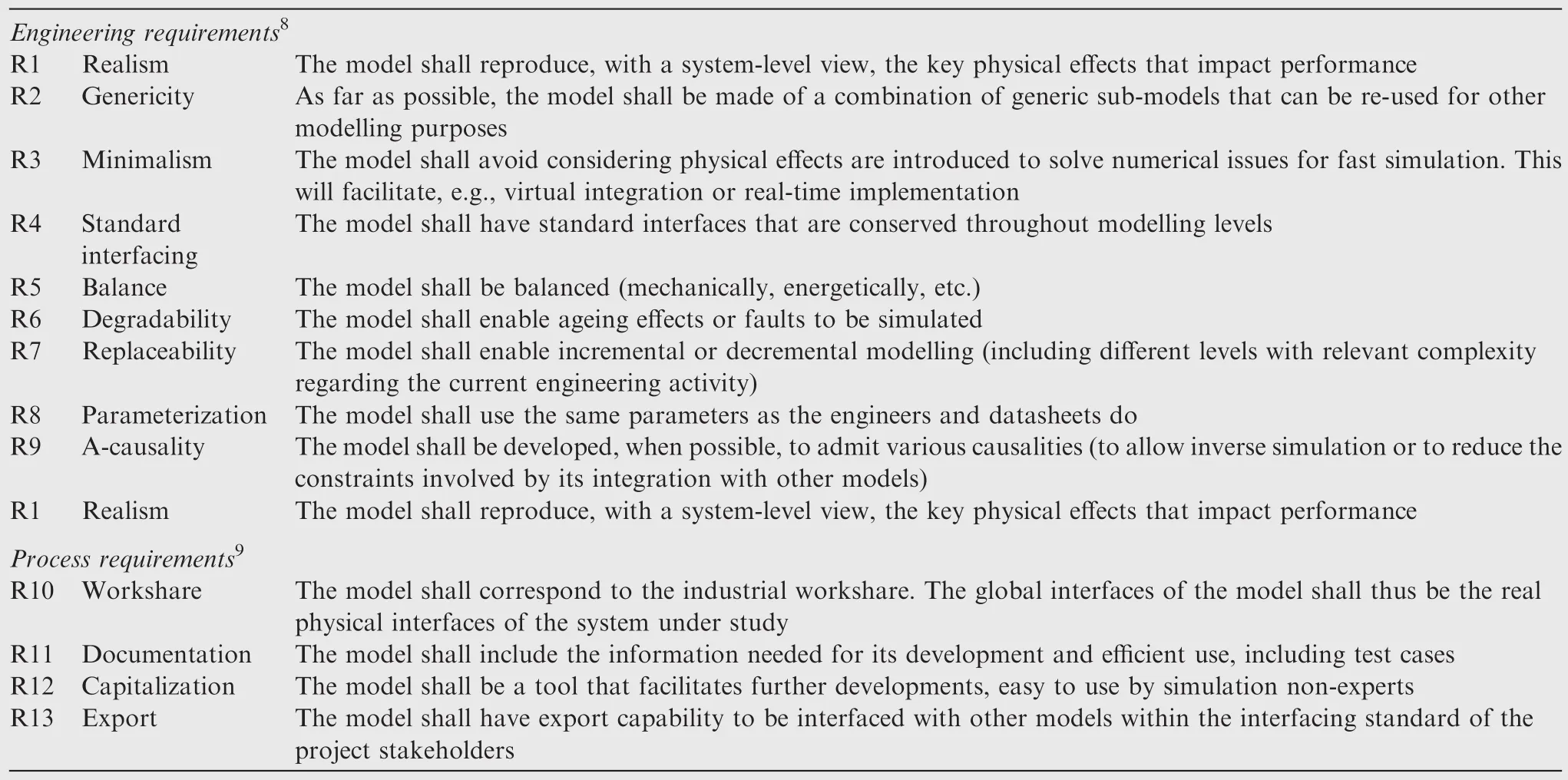
Table 1 Proposed generic model requirements.

development process,progressing from a top view to a very detailed view.It has many practical advantages:

-M&S debugging is easier as the simulation software is used with progressive levels of complexity.

-The model’s developer can perceive the contribution of each modelled effect when it is added into the model and therefore increase his understanding of the system’s behavior.

-At each step of the process,few additional parameters have to be introduced.

However,this approach may require some experience regarding the order to be used to progressively introduce the considered effects.Analysis of the contribution of a given effect to performance can be biased by its combination with already introduced effects.

3.1.2.Bottom-up(or decremental)approach

The full model is developed directly,and then progressively simplified if necessary.All the complexity is introduced at the same time,requiring numerous parameters and functions or submodels of the simulation software.Unlike incremental modelling,it deprives the model’s developer of the opportunity to feel the individual contribution of functional and parasitic effects.However,this approach is well suited to the needs of virtual prototyping,e.g.for achieving a reduced-order control model,real-time implementation,or integration in large system models,in particular when the system to be modelled is already defined in detail.Although this approach introduces all the complexity at the same time,there is a natural temptation to adopt it during product development,with the intention of being able to draw rapid advantage from the numerous submodels available in the simulation software libraries.However,it can be observed that this solution is often used implicitly out of facility:it is not driven by the objective of meeting the M&S needs,but rather to try to compensate for a lack of knowledge(at both process and physics levels).

3.2.Modelling levels

Whatever the approach adopted(incremental or decremental),the structuring of model libraries requires modelling levels to be defined.Thus,the number of the model of a given object does not grow exponentially,and simulation speed and fidelity can be balanced for a given engineering activity.

3.2.1.Level per model refinement

A simple solution is to limit the number of modelling levels to,e.g.,3:basic(to support top level decisions),normal(for sizing and control design)and advanced(for virtual prototyping).A more structured approach is found by considering 4 levels as proposed5for application to aircraft electrical power systems,in Fig.1.5

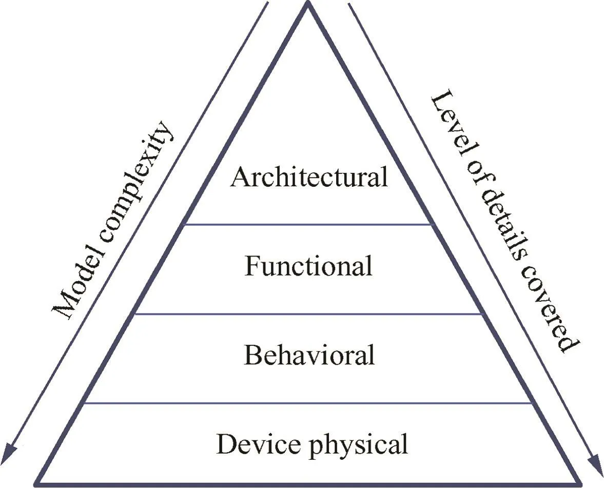
Fig.1 Modelling levels.5

#a1 Architectural level.This level enables global architectural studies.The model involves Boolean states and control logic with steady-state solutions and idealized control loops.

#a2 Functional level.This level typically introduces low frequency dynamics.The model reproduces the system and subsystem control structure in detail and is suitable for linearization.

#a3 Behavioural level.Lumped-parameter models are introduced to increase the range of frequencies reproduced by simulation,while transistor switches are considered as ideal.

#a4 Device physical level.This is used for modelling a particular device with a more physical view including multiphysics coupling and parasitic effects.

3.2.2.Level per numerical complexity

Another approach,as selected in the European project Actuation 2015,10is driven by numerical complexity.Five modelling levels are defined with respect to the computational load and the model’s ability to be inverted:

#b1 Perfect.Models are linear and only address functional effects.There is no parasitic effect.

#b2 Linear and invertible.Parasitic effects are introduced in a way that keeps the model linear and invertible.

#b3 Non-linear and invertible.Functional and parasitic(soft)non-linearities are introduced in a way that keeps the model invertible.

#b4 Hard non-linear.Non-linearities are modelled in a more realistic way that triggers a few state events.

#b5 Fully switched.Non-linearities are modelled without restriction and the model generates numerous state event triggers.

Other options exist,e.g.focussing on the level of abstraction:functional,signal,network (physical with lumped parameter models) and geometrical (physical with distributed-parameter models).In practice,any decomposition into levels is explicitly or implicitly linked to engineering tasks,product decomposition,modelled effects and numerical complexity.All these examples illustrate the challenge of sharing a common view of the modelling levels.There is obviously no single solution,given the variety of standpoints:engineering activity(architecting,sizing,integration,verification,etc.),product(system,subsystem,equipment,component,device),etc.This difficulty is magnified for power transmission and motion control systems.Firstly there are numerous nonlinearities that play a significant role in performance(e.g.backlash,friction,volume and pressure dependent hydraulic compliance,etc.).Secondly,there are many dynamics that range over decades (e.g.hydraulic/mechanical/electrical/thermal time constants)and that combine with high frequency switching(e.g.sampling of digital control,switching of power electronic devices,porting of hydraulic motors and pumps).

Of course,a given simulation can mix submodels having different levels,according to the current engineering task.This emphasizes again how important it is to meet the requirements relative to model interfaces(requirement R4)and replaceability(requirement R7).

3.3.Model architecture

Although it often attracts little interest,model architecting is an important step towards meeting the requirement R10(workshare).It should be kept in mind that a given modelling activity is only a through point and part of a whole project.Therefore,continuity of the models between the different phases of a product’s life cycle is an important enabler of industrial and economic efficiency.This is why any effort to facilitate the understanding and reuse of the model among project stakeholders undoubtedly increases the efficiency of the simulation-aided process.Adopting an architecture at model level that is similar to that the real product extends the sharability of model simulations(e.g.for virtual verification of a product element or for product virtual integration).In some particular cases,this idea can even make the model representative of the geometrical topology of the real product.This is illustrated by Fig.2 for the case of use of a linear electromechanical actuator(demonstrator of helicopter main rotor actuator).11The main idea here is based on the combination of bodies(e.g.driveshaft or rod)that are linked by joints(e.g.hinge or prism pair),power transmission devices(e.g.electric motor,brake or nut-screw)or even sensors(not mentioned on the figure for the sake of simplicity).This idea is starting to be implemented in some commercial tools that enable CAD models to be directly imported into the lumped parameter simulation environment(e.g.for hydraulic lines in AMESim).

3.4.Modelled effects vs.modelling needs

One major difficulty in model development is related to the selection of the effects to be considered or neglected.The choice depends on the current engineering task to be supported in the most efficient manner through M&S.For this purpose,Fig.3 proposes a matrix view of the links between the needs and the modelled effects,using the example of an electromechanical actuator.12,13The first column lists the potential effects or parameters to be considered,while the first line lists the engineering activities.It is worth noting that the last 4 columns provide indicative information related to the complexity of the model development and its implementation(number of parameters and state variables,computational load and related time constants).The matrix is then filled to indicate whether introducing the effect is mandatory(Y)or simply welcome(P)for the activity considered.

This matrix view is of particular interest when the intention is to define a minimal set of models that are consistent with the chosen modelling levels.Last but not least,it can also be employed to formalize the analysis of a commercially available library prior its use.

3.5.Model balancing

It seems obvious that models should be balanced(requirement R5).However,this is rarely ensured in the libraries of commercial simulation environments.This shortcoming deprives the engineers of efficient ways to expand the scope of simulation and consequently to address wider tasks.The following two examples illustrate the interest of making the models balance at energy and mechanical levels quite well.

3.5.1.Energy losses

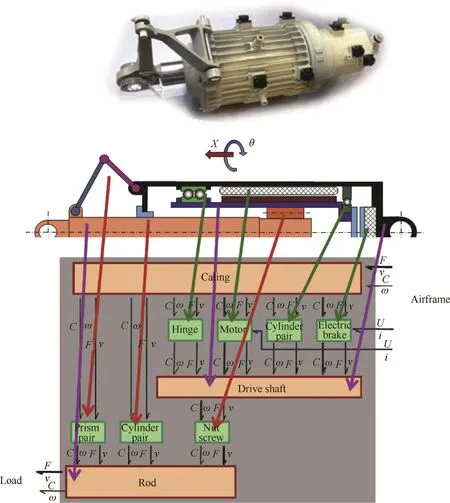
Fig.2 Illustration of model architecting using the example of an electromechanical actuator.11

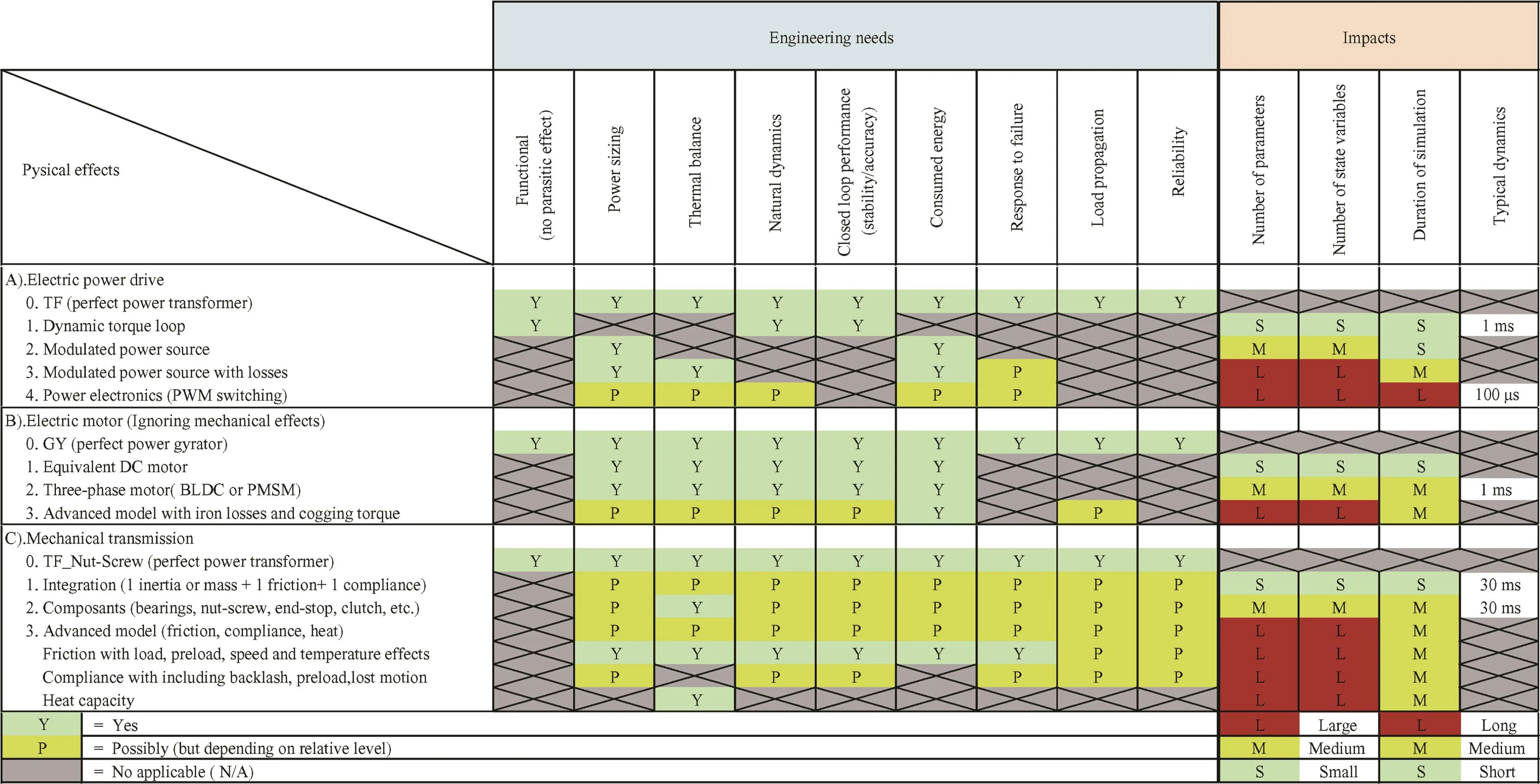
Fig.3 Proposal of a matrix view of the link between engineering activity and modelled effects,using the example of an electromechanical actuator,adapted from Refs.12,13.

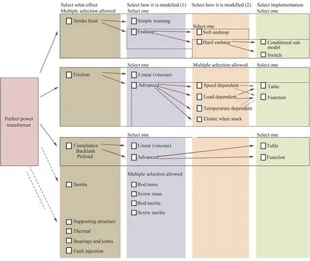
Fig.4 Simplified example of model customization from generic submodels.

Any energy loss(e.g.friction in bearing,resistance of motor windings,switching losses of power electronics)should be viewed as a source of heat that flows at a thermal port(heat power output).This power port potentially allows the model to be made sensitive to temperature,and consequently enables it to reproduce the thermal snowball effect.In an EMA,a temperature rise of 100°C increases the resistance of motor copper windings by 40% and reduces the induction of motor samarium-cobalt magnets by 4%.This requires higher drive current to generate the same electromagnetic torque,which,in turn generates more heat.The same type of example can be given for hydraulic actuators:mechanical and volumetric efficiencies are directly linked to the oil viscosity,which may change by a factor of 130 when the fluid temperature changes by 100°C.

3.5.2.Mechanical reactions

Ideally,any mechanical model should be balanced in the 3 translational and the 3 rotational directions.As an example,it is considered a parallel-axis spur-gear reducer having a speed ratio ofNbetween the input and output shafts.In steady speed conditions,the structure supporting the reducer body should withstand the reaction torque,which isNtimes the drive torque(the sign depends on whether or not the input and output shafts rotate in the same direction).Therefore,introducing a mechanical port for the holding structure is interesting,e.g.for sizing the anchorage or for running dynamic analysis considering the anchorage compliance.Mechanical balancing may be implemented only partially to avoid unnecessary complexity(full mechanical balance may lead to a model with 6 degrees of freedom if forces and torques are considered in the three spatial directions).For example,the common model of a bevelgear reducer considers only motion and force at the input and output shafts(1-D model where the considered spatial direction changes among the power paths).Partial mechanical balance can be implemented at torque level to determine the reaction torques at the supporting frame in the two directions of the reducer shafts.

Note:Taking a long-term view of the model’s use requires relative motion to be considered in mechanics.e.g.for a perfect reducer of ratioN,the speed ratio should apply to the shaft velocity relative to the housing,and not to its absolute veloc-ity.In this case,attention should be paid to making inertial effects apply to absolute,not relative,acceleration.

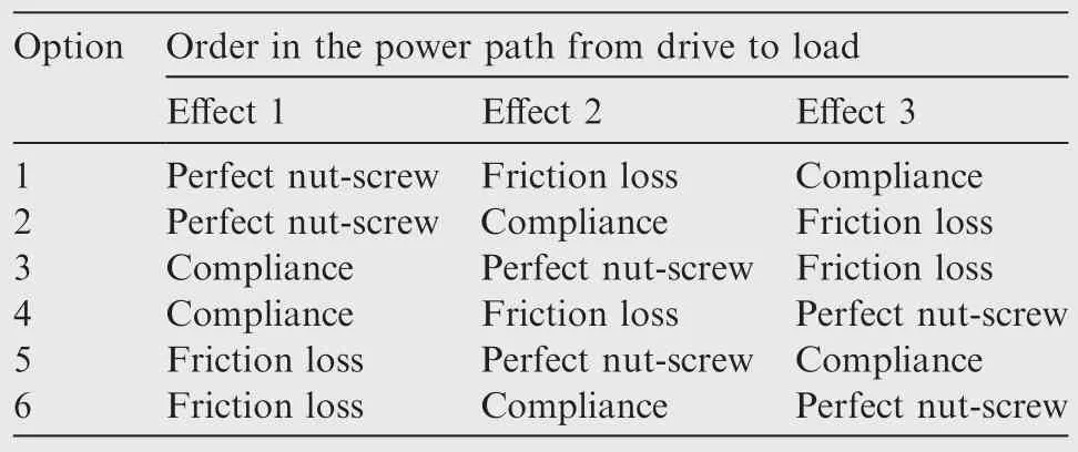
Table 2 Candidate locations of compliance and friction effects in a nut-screw model.

3.6.Order of effects in the power path

Modelling lumped parameters requires choosing where each considered effect is located in the power path from drive to load.When this effect is distributed in practice(e.g.compliance or inertia of a rod,or pressure loss in a pipe),the choice made simplifies the model but introduces a loss of realism.Unfortunately,there is not a single,unique possibility for locating the distributed effect with a lumped standpoint.This is illustrated by Table 2 in the case of a nut-screw,where parasitic friction and compliance are each introduced once.The option chosen impacts both static and dynamic responses of the modelled system.However,there is not a general rule and the choice may vary according the current engineering need,based on the experience of the model designer.

Notes:

-A very small number of references,e.g.Ref.14,report and highlight the impact of choosing the location of the effects considered.These effects are generally ignored.

-Location of effect is even important when a friction model is made of two parts,e.g.for modelling mechanical power transformers:a load-dependent and a load-independent friction.The calculated friction force may be strongly affected by the order chosen for the two effects(as well as the side of the model used to calculate the power quadrant),see Section 3.4.

4.Model implementation

4.1.Signal view vs.power view

Two generic perspectives can be adopted to implement a model of a controlled power transmission system:a signal perspective and a power perspective.

4.1.1.Signal perspective

The signal perspective comes from the times of analogue simulators that became available during the 1960s.The differential equations found in the modelling phase were implemented by manual connection(like telephone switchboard operators do)of physical units(the blocks).Each block performed either amplification,integration or summation functions.The blocks were first made using vacuum valves,then transistors and finally integrated circuits.This approach was later replicated when simulation software was introduced.

Using this block-diagram approach is attractive because any model can be implemented,as long as the set of generic blocks provided in software libraries is sufficiently large.Moreover,this approach is identical to the one commonly used to represent signal flows in signal processing and control,making for continuity in both signal and power models.

However,these advantages are balanced by various drawbacks.First,readability is very poor:a power flow requires two signal flows,e.g.voltage and current,or force and velocity.Second,a power flow can be inconsistently modelled with block diagrams:e.g.forgetting one of the two equations of a pure power transformer,or using different parameters for each equation.Third,everything has to be done,including dealing with numerical stability,in particular in the presence of hard discontinuities(e.g.for endstop or friction):the designer wastes time developing and setting up models instead of focussing on his engineering activity.

4.1.2.Power perspective

The power perspective uses power connections between model elements whatever the level(product level:component/equipment item/system,etc.,or abstraction level:function,basic physical effect,etc.).Therefore,a single connection passes the two variables,the product of which gives the power flowing between the connected elements.These elements replicate the power flow and the physical connections at their boundaries.The power perspective is supported by two generic graphical representations:circuit(or network)and Bond-graph.15The first one uses through and across variables,while the second one uses effort and flow variables.At a higher level that combines a lot of basic effects,icons can be used to display the simulated device more synthetically.Besidethe improved readability of the model,this approach draws benefit from the re-use of capitalized models(verified,documented,updated),thus accelerating implementation of the model.The main drawback comes from the risk of associating elements or icons without taking time to understand what effects are modelled or ignored.This naturally leads the user to develop models that are too complex with respect to the current engineering need,with a bottom-up approach(see Section 2.1.2).Also,versatility may not be sufficient if the existing elements cannot be customized(e.g.outputting an internal variable or introducing a new input to improve the model’s fidelity).

The readabilities of the two approaches are compared in Fig.6.In practice,commercial simulation software tends to offer the two approaches in order to enable both signal and power flows to be combined.

4.2.Progressive construction of the model

The matrix view suggested in Section 3.4,can be employed efficiently to customize the development of supermodels from generic models.This is illustrated by Fig.4,using the example of a nut-screw mechanical transmission.

The first step consists of selecting what effects are to be considered.The second step enables the user to select how the considered effect will be modelled.The third choice indicates in what way the model will be implemented.The model is automat-ically constructed according to the checked boxes.The configuration can be saved and associated with a given engineering activity for direct reuse of the supermodel for future similar tasks.The example of the nut-screw is highly illustrative.Beside the perfect power transformation effect,friction,for example,can be considered(what effect).Then the type of friction model can be selected(how to model),e.g.advanced model including effect of speed,load and temperature.Then,the way the model is implemented can be selected(what way).For this step,transition between sticking and sliding can be managed e.g.using a hyperbolic tangent function,a reset integrator,etc.16

Notes

-The numerical management of the sticking/sliding transition may be achieved by introducing some additional effects(e.g.compliance of the contact before sliding)although they were not intentionally considered.

-Another step can be introduced in the construction of the supermodel,dealing with how the model is parameterized(see Section 3.5).

-Defining the model’s interfaces to enable replaceability

requires a view anticipating the different evolutions of the model.This deals,in particular,with the introduction of ports ensuring that the model is balanced(see Section 3.5).Some commercial simulation environments already offer features to conditionally enable model parts or to replace a submodel by another one.However,the implementation of the proposed progressive model construction is still restricted.For example,the parameters’window cannot be shaped dynamically as a function the selected effects,model type and implementation.

4.3.Types of models

There are different ways to define the types of models.

4.3.1.By purpose

Knowledge models are obtained from science,which provides a mathematical equation describing a conservation principle(e.g. momentum, energy, mass, current, etc.) and transformation/storage/dissipation of energy(e.g.nut-screw,inertia and friction).In the domain of actuation,these models quickly become non-linear and high-order.Representation models are identified from measurement,generally without resort to any physical consideration(e.g.polynomial representation of a worm gear friction loss,or equivalent second order of a servo valve).Representation models are generally simple and low order.Control models are employed for the synthesis of controllers.Most of the time,they are linear and low order,being obtained through identification from tests or reduction/-linearization of knowledge models.Surrogate models and metamodels17are mainly used as a very simple way to consider the dominant and coupled characteristics that impact preliminary sizing and optimization.Real-time models balance realism and low computing load for SIL or HIL simulation.

4.3.2.By formalism

Among the different types of models(Mathematical,2-D drawing,3-D views,circuits,diagrams,Bond-graph,charts,tables,scale,etc.)system-level simulation usually mainly involves mathematical models.Diagrams and networks serve for graphical user interfacing.Circuit or network representations are of huge interest when they use standardized symbols,if they exist for fluid power18or for electrical and electronic diagrams.19

4.3.3.By mathematical form

When the mathematical formalism has been chosen,the mathematical form of the model is strongly linked to the effects considered and the intended use of simulation:linear/non-linear,static/dynamic,constant/variable parameters,continuous/discrete time,continuous/discrete values,deterministic/stochastic,lumped/distributed parameters,etc.Unfortunately,the usual names used for defining the type of model(0-D,1-D,3-D,etc.)are insufficiently accurate.For example,3-D can be associated with 3 directions of space but also with distributed effects,time effects being or not being considered.With this name,a 3-D model can,for example,be a static model of a spatial multibody system with lumped compliances and inertia,e.g.landing gear kinematics.It can also correspond to a dynamic model of the same landing gear with distributed mass and compliance effects.To make the model types more accurate,three types of information are proposed to define them:

-1-D,2-D,3-D to define how many spatial directions are addressed simultaneously.

-Static(s)or dynamic(d)model according to whether time is ignored or not(leading to Algebraic Equations(AE)or differential equations(DE)).

-Lumped(l)or distributed(d)parameters,leading to ordinary differential equations(ODE)or Partial Differential Equations(PDE),if time is considered.

According to this proposal,a 3-Dsl model is 3-dimensional,static and considers lumped-effects.

Notes

-Models can also be called black,grey or white.However,meanings can vary slightly.Generally,white models are associated with knowledge models while black models relate to representation models.However,black model is also used to define a knowledge model that has been encoded to prevent the user from accessing the model’s equations and their implementation.

-Knowledge and representation models are also called deductive and inductive models,respectively.20

4.4.Causalities

Causality relates to the definition of the cause(s)and consequence(s).For real systems,causality is easy to define at functional level.E.g.a flight control actuator aims at positioning the flight control surface(the consequence)in response to the position setpoint generated by the flight control computer(the functional cause)and to the aerodynamic load acting on the surface(the disturbance cause).In M&S,the causality,i.e.the definition of input or output type for a given variable)depends on the standpoint,which is closely linked to the engineering phase(see Section 1).This is illustrated in Table 3,in the case of a nut-screw.

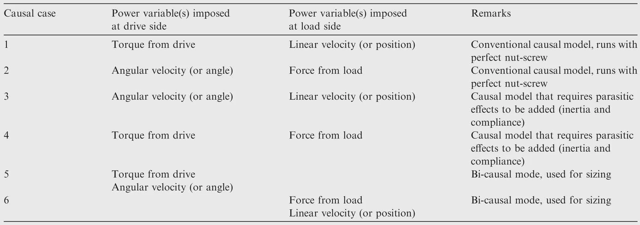
Table 3 The six causal cases considering power variables for a nut-screw transmission(supporting structure assumed fixed).

The first two lines correspond to the conventional causality where one power variable(force/torque or linear/angular velocity)is imposed at each side of the nut-screw.This is representative of the functional flow of power variables that is reproduced for virtual testing(cf.Section 3.1.1).Lines 3 and 4 also define a causal use of the model but in a nonconventional way that requires parasitic effects to be introduced in order not to lose consistency between inputs.Lines 5 and 6 are relative to sizing(cf.Section 3.1.3),where both power variables are imposed on a given side of the nutscrew:this is the bi-causal use of the model.

Common simulation environments implement causal models only.They impose hard constraints in the development of the model,in particular for reuse and model integration.Avoiding algebraic loops and numerical derivations generally requires a given model to be implemented in multiple causal cases(e.g.lines 1-4 of Table 3)to keep model connectivity with respect to considered effects(requirement R9).

Recent years have seen the emergence of non-causal modelling languages21that can potentially generate the simulation code for any causal case,including bi-causality(as long as the model is not under-or over-determined).In simple cases,they are even able to make formal manipulations and to cope with the presence of algebraic loops and numerical derivations,which cannot be avoided for bi-causal simulation.

Notes

-A-causality could be better exploited in non-causal simulation environments.Instead of considering causality at the level of power variables only,non-causal models(e.g.lines 5-6 of Table 3)could be used to output control or internal variables in power transmission systems:e.g.displacement of a compensated hydraulic pump,duty cycle of a power electronics inverter,control current of a servovalve,etc.Unfortunately,this way of using the libraries of commercial non-causal simulation environments is not directly available and still requires the models to be modified.

-The availability of non-causal modelling and simulation environments should not be interpreted as the removal of all constraints concerning model development and implementation.This is another motivation to develop,disseminate and apply best practices.First,avoiding algebraic loops and derivations,as is generally required in causal simulation,makes the model’s simulation faster and/or more accurate.Second,for a given level of detail,a model may not be invertible in all cases.For instance,when friction is modelled without contact compliance and is used to reproduce true sticking,it is impossible to calculate the external forces in stuck conditions.Indeed before breakaway,friction opposes external forces to avoid motion:the model is under-determined.

4.5.Parameterization

Parameterization plays a significant role in the added value generated by M&S.The example of friction is once again very illustrative.In the IEEE community, friction is mainly considered as speed dependent because this serves the control designer’s needs well:being linear,the basic viscous friction model facilitates dynamic analysis and control synthesis.Then the model is progressively enhanced,introducing Stribeck and Dahl effects to make a virtual prototype.Load and temperature effects are rarely considered.In the mechanical domain,friction is mainly considered as load dependent,using mechanical efficiency because it meets the power sizing need well.This view is also shared by the suppliers of mechanical transmission devices.However,the data are generally incomplete,in particular concerning operation under aiding-load or at low velocity.22

There are,in fact,various ways to parameterize a model.Fig.5 illustrates how a data flow can be represented.It highlights how the parameters required by a nut-screw model can be calculated from available parameters.It can be seen that friction losses are modelled using direct and indirect efficiencies.These parameters can be either obtained directly from suppliers or calculated from the friction coefficient and the helix angle(depending on pitch and base diameter).Another interesting suggestion present in Fig.5 is the use of a single parameter to quantify backlash or preloading(using negative backlash).In that simple manner,the backlash parameter can be varied to address the performance robustness against,e.g.,accumulated service or increased friction.Not represented in the figure,the friction force can additionally be made sensitive to preload.22

Useful information for each parameter involved in the model can also be introduced on the basis of the author’s experience.A parameter table is generated in order to improve traceability and capitalization.It includes:

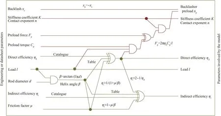
Fig.5 Example of parameterization of a nut-screw model.

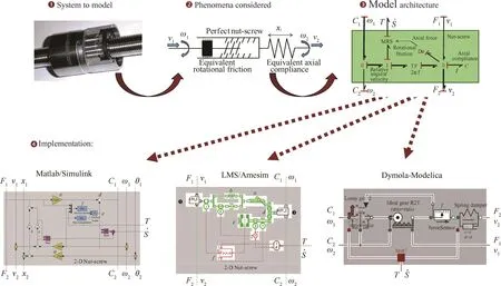
Fig.6 Example of platform-independent development of a nut-screw model.

-A text indicating the source of information that provided the numerical value to be used(e.g.document or email reference).

-A letter indicating the type of source of information,e.g.R for requirement,A for assumption,D for design choice,S for supplier data sheet,H for hypothesis,etc.

-A cell colour indicating the uncertainty of the parameter,e.g.from red for highly uncertain(most of the time for dissipative effects),to green for very low uncertainty(e.g.density of spring steel).

4.6.Model implementation

When possible,it is interesting to make the model independent of its implementation in the intended simulation environment.This allows the model to be implemented by each project stakeholder whatever the simulation platform in use in his company.An illustration is provided in Fig.6,again using the example of a nut-screw system,with a mechanical quadriport point of view(rotation and translation at both nut and screw).The physical effects to be considered for the real nutscrew system and their arrangement are defined in a first step using simple schematics(or circuit representation).From drive to load sides,friction is firstly introduced in the rotational domain,followed by perfect power transformation and finally compliance in the translational domain(option 5 of Table 2).The corresponding Bond-graph is then built to define the model structure and its internal and external causalities(causal case 3 of Table 3).The presence of the heat port and the mechanical quadriport allow the model to be balanced mechanically and energetically.Finally,the model is implemented,according to the information provided by the Bondgraph,in the Matlab-Simulink,AMEsim or Dymola environment.Friction is reduced at rotational level and made sensitive to speed,axial force and temperature.There is no particular difficulty in replacing the linear model of compliance with a more advanced one including preloading or backlash.8

4.7.Modelling and simulation desk

The broad offer of commercial simulation environments provides a huge set of tools enabling engineers and researchers to address more and more extensive engineering domains without writing a single line of code,including for linking 1-D and 3-D models.The M&S desk can be represented by Fig.7,which defines two circles:

-The global view(internal circle)involves lumped parameter models that couple fluid power,rigid multibody systems,electronics,etc.and control design.

-The local view (external circle)deals with distributed parameters and couples Finite Element Models(FEM)for solid mechanics,Computational Fluid Dynamics(CFD)for thermo- fluidics and 2-D/3-D electromagnetics.

Links between local and global views can be established in both directions depending on the engineering activity,in particular with the development of model interfaces standardization,e.g.FMI.For system level M&S,the local view can,for example,generate tables or metamodels to decrease model complexity by reducing the distributed effects to their loworder lumped parameter equivalent.Co-simulation or import/-export functions are now well established to simulate global and local models simultaneously,when necessary.23

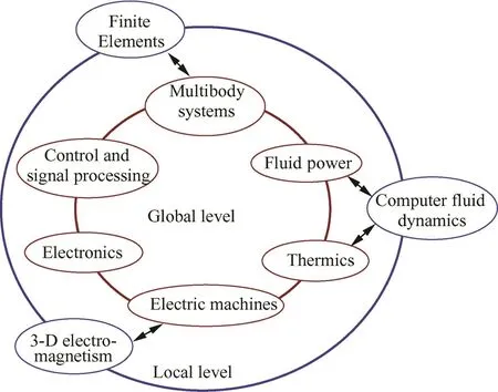
Fig.7 Virtual prototyping environment.

4.8.Model verification and validation

Model verification(see definition in Appendix A)is a very demanding task during the development of high fidelity models,in particular for mechanical transmissions,which display hard and numerous non-linearities and discontinuities.Sufficient time and effort has to be allocated to the model verification task(e.g.for electromechanical actuators24),which has to prove the correct implementation and running of the model,for the whole range of parametrization(including for model excitations).The case of friction in mechanical transmissions again provides a good illustration.The friction force depends on velocity,transmitted force and their combination through the power quadrant of operation(aiding or opposite load).Fig.8 gives a proposal for a mission profile(e.g.velocity of drive and force applied by the load)that verifies all possible transitions in sliding mode.

Like model verification,model validation(see definition in Appendix A)is expensive and time consuming.However,major considerations have to be kept in mind for extensive use of M&S:

-Validation of submodels(or partial validation)does not always allow all model parameters to be identified.In this case,validation of the model may still require an identification step first.However,the model has to be validated without any change in its parameters for the whole domain of operation to be covered.

-Model validation requires specific real tests that are generally very different from performance tests.The validation test program has to be specifically built in order to validate the model fidelity step by step,with judiciously chosen excitations and observations.

-In the most efficient situation,simulation and experiment should progress simultaneously:real tests suggest improvements to the model in specific directions,while model parameterization points out the need for real tests to identify uncertain effects or parameters.Unfortunately,it is rarely possible to run this process in large companies that have to plan the use of test-benches up to one year in advance.

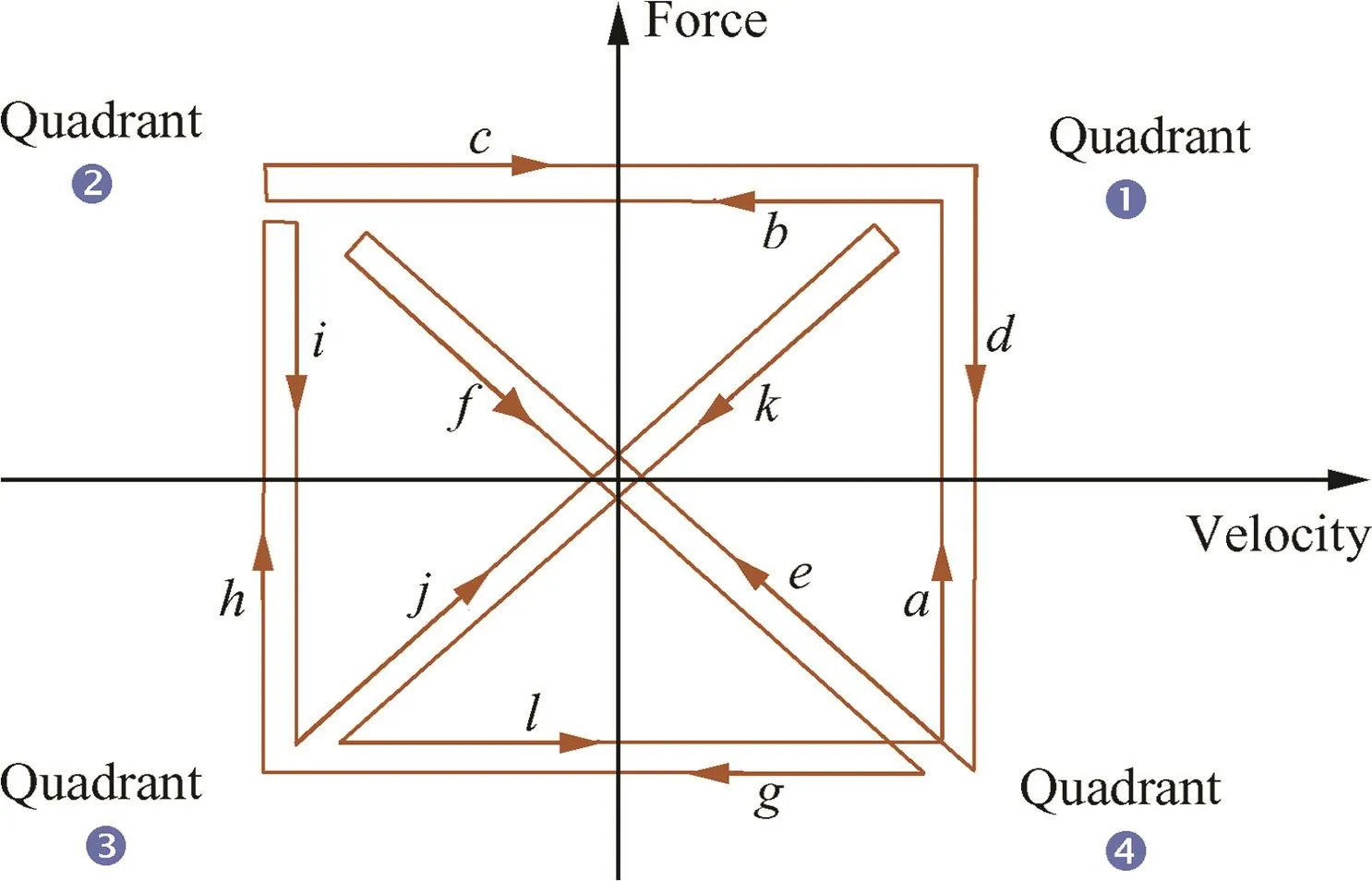
Fig.8 An example of mission profile for verification of a friction model.

-The skills of real test engineers make them particularly efficient for model validation activities and for virtual testing.The replacement of real tests by hybrid and ultimately virtual tests will not make test engineers disappear,but simply evolve.

It has been frequently observed that model verification and validation,and the related documentation,are generally considered as boring tasks although they should be seen as a major through point for model-based and simulation-aided design.In practice,three activities,with their time,budget and workforce allocation,are often missing in projects involving intensive M&S:model integration,model validation and model documentation(including references and test cases).

5.Conclusion

Today’s offer of commercial software for modelling and simulation is huge and covers ever-broadening needs.Progressively,the physical effects are modelled with increased realism while numerical issues and limitations tend to disappear.Consequently,the main difficulty does not come from the ability of the simulation tools to meet the needs;each product is globally capable of addressing similar M&S problems.The main challenge deals rather with the ability of the persons involved in the M&S process to make profitable,capitalized and time efficient use of the existing simulation concepts and tools.This consideration has motivated the present review and suggested best practices for the development,implementation and use of system-level models.Simple examples have been provided to illustrate how the proposals can be put into practice.Viewing the model as a product in itself and adopting standards addressing its whole life is an attitude that has just started to spread.Great efforts still have to be made to rise to the challenge and to converge towards a uniform view,in order to facilitate the acceptance of M&S for qualification and certification in the near future,whatever the product domain,level and engineering activity.

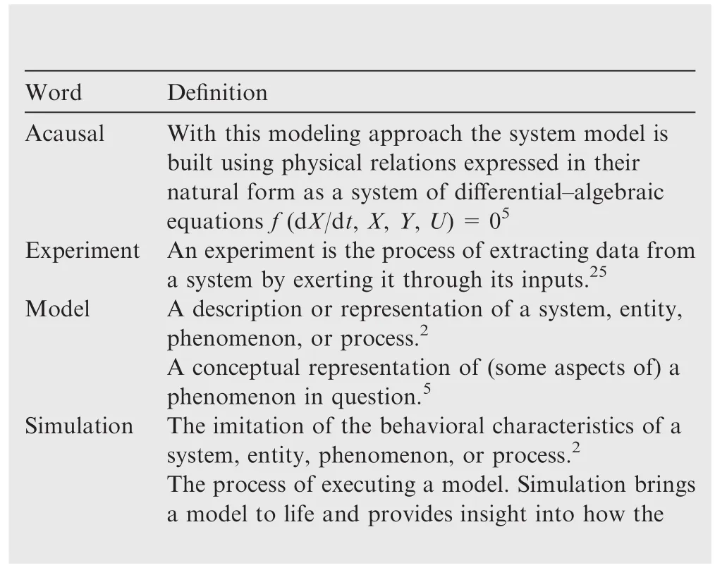
Appendix A.Useful definitions

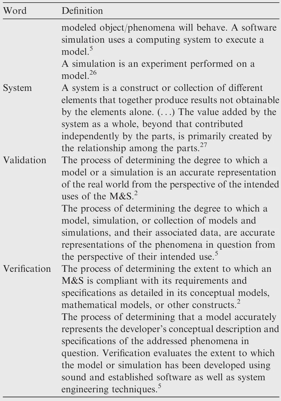
Appendix A(continued)