Neural-Network-Based Terminal Sliding Mode Control for Frequency Stabilization of Renewable Power Systems

Dianwei Qian and Guoliang Fan

Abstract—This paper addresses a terminal sliding mode control(T-SMC)method for load frequency control(LFC)in renewable power systems with generation rate constraints(GRC).A two-area interconnected power system with wind turbines is taken into account for simulation studies.The terminal sliding mode controllers are assigned in each area to achieve the LFC goal.The increasing complexity of the nonlinear power system aggravates the effects of system uncertainties.Radial basis function neural networks(RBF NNs)are designed to approximate the entire uncertainties.The terminal sliding mode controllers and the RBF NNs work in parallel to solve the LFC problem for the renewable power system.Some simulation results illustrate the feasibility and validity of the presented scheme.

I.INTRODUCTION

W ITH the rapid development of economy,electrical power demand has become continuously stronger year by year.A vast amount of fossil fuels utilized in power generation results in energy crisis and environmental deterioration around the world[1].One possible solution is to adopt clean and renewable energy instead of fossil fuel for power generation.Wind power is now the fastest growing energy source around the world because of its zero emission[2].The percentage of wind generation in power systems increases with years.Wind energy has become one of the central research themes in energy science.

Concerning real applications,a constant supply of electricity in some remote areas cannot be guaranteed by power grids.In these areas,wind energy may be inexhaustible and convenient.Therefore,wind power has been paid more and more attention and some control problems rise up in power systems with wind turbines[3].An advocacy of wind power is due to its sustainable and renewable status.However,wind power affected by climate changes is intermittent.Its intermittence also has impressive effects on operation and control of renewable power systems.

Consider a power system with wind turbines.The load in the power system is random and the power output of wind power is fluctuating.The power-output fluctuation and the load change would pose a reliability supply challenge.The challenge is displayed by power imbalance and frequency deviation in the power system[4].Consequently,frequency control strategies must be adopted to overcome the challenge.

Load frequency control(LFC)is one of the most profitable auxiliary services to guarantee the stable operation of power systems with the objective of preserving the balance between power generation and power consumption[5].Recently,the LFC problem of renewable power systems has been paid more and more attention[6],[7].In order to attack the generation intermittency of renewable power systems,some LFC methods have been investigated,such as fuzzy control[8],[9],predictive control[10],[11],and adaptive control[12],[13].

Invented by Utkin,the sliding mode control(SMC)is recognized as a powerful design tool[14].On the sliding-mode stage,an SMC system is completely insensitive to parametric uncertainties and external disturbances under certain matching conditions,which exhibits better performance than the conventional robust control methods[15].This property inspires some researches on SMC for the LFC problem[16]−[22].However,the SMC-based LFC methods in pervious works[16]−[22]do not consider the complexity and challenge of renewable-energy sources.The method of terminal sliding mode control(T-SMC)[23],[24]guarantee the convergence of the SMC system within finite time.The T-SMC method can be considered for the LFC problem of renewable power systems.

Power systems are inherently nonlinear[25].The two main nonlinear factors are the governor dead band(GDB)and the generation rate constraint(GRC).The existence of GRC has adverse effects on the system robustness,the system performance as well as the system stability[26].A common technique to deal with the GRC nonlinearity is to design a controller for the linearized nominal model;then the controller is directly imposed on the original nonlinear system.In a sentence,the linearized model is adopted to achieve the control design for the original nonlinear system.Although it is available in most cases,the technique has some potential hazards because there is no theoretical guarantee on the stability of the control system.Concerning the applications of SMC on LFC[16]−[22],some works[16],[17],[21]only consider linear power systems and other works[18]−[20],[22]adopt the linear-model-based design.However,a series of drawbacks may be induced to the linear-model-based control systems because of lack of theoretical supports.

The methodology of radial basis function neural networks(RBF NNs)has a universal approximating feature[27].The RBF NNs technology has been widely adopted to solve nonlinearities and uncertainties of complex systems[28].In[20],RBF NNs are employed to approximate and compensate the GDB nonlinearity of power systems.However,how to conquer the GRC nonlinearity by RBF NNs remains untouched and problematic.To turn the T-SMC into practical accounts on the LFC problem of renewable power systems,it is urgent to solve the GRC nonlinearity by the RBF NNs technique.

This paper focuses on the T-SMC method for LFC of nonlinear power systems with wind turbines.To deal with the GRC nonlinearity,the linearization method is adopted at first.Then,a terminal sliding mode controller is designed based on the linearized nominal system.The uncertainties of the LFC problem have three components,i.e.,the intermittency of wind power,the uncertainties of power systems and the error of linearization.The components mix together and worsen the uncertainties of the LFC problem.To theoretically guarantee the system stability,the sliding-mode-based neural networks are designed to suppress the entire uncertainties.Weight update formulas of the neural networks are derived from the Lyapunov direct method.The neural-network-based T-SMC scheme is employed to accomplish the LFC problem.To illustrate the feasibility and validity of the presented scheme,some numerical simulations are conducted by a nonlinear interconnected power system with wind turbines.

The remainder of this paper is organized as follows.Section II formulates the system configuration.Section III presents the T-SMC method,the RBF NNs design and the system stability.Simulation results are demonstrated in Section VI.Finally,conclusions are drawn in Section V.

II.SYSTEM CONFIGURATION

A.Component Dynamics

This paper considers the LFC problem of a multi-area interconnected power system.The power system is composed of N control areas which are interconnected by tie-lines.Fig.1 represents the block diagram of the ith control area in the multi-area power system.In Fig.1,variables∆Pgi(t),∆Xgi(t)and∆fi(t)are the incremental changes of generator output,governor valve position,and frequency,respectively.∆PLi(t)is the load disturbance,∆Pci(t)is the control input.Tgi,Ttiand Tpiare the time constants of governor,turbine and electric system governor,respectively.Bi=1/Ri+1/Kpiis the frequency bias factor where Riis the adjustment deviation coefficient and Kpiis the electric system gain.Tijis the synchronizing power coefficient between area i and area j,i,j=1,...,N and N is the number of control areas.

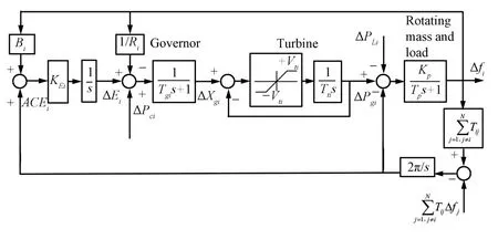
Fig.1.Dynamic model of the ith control area of the multi-area interconnected power system concerning GRC.

According to the LFC objective,not only should the frequency of the control area return to its nominal value,but also the net interchange through the tie-line should return to the scheduled values.To achieve the composite goal,a measure,named area control error(ACE),is introduced.In Fig.1,the measure in the ith control area is defined by

where∆Ptie,i(t)is the tie-line active power deviation,determined by

where∆Vi(t)is employed to represent the control area interface,defined by

To force the composite measure(1)to zero,the integral of ACEi(t)is used as an additional state,determined by

where KEiis the gain of this additional state.

Define a vector xi(t).The vector is described by xi(t)=[∆Xgi(t)∆Pgi(t)∆fi(t)∆Ptie,i(t)∆Ei(t)]T.Then,the following state equations can be deduced from(1)−(4)and Fig.1.

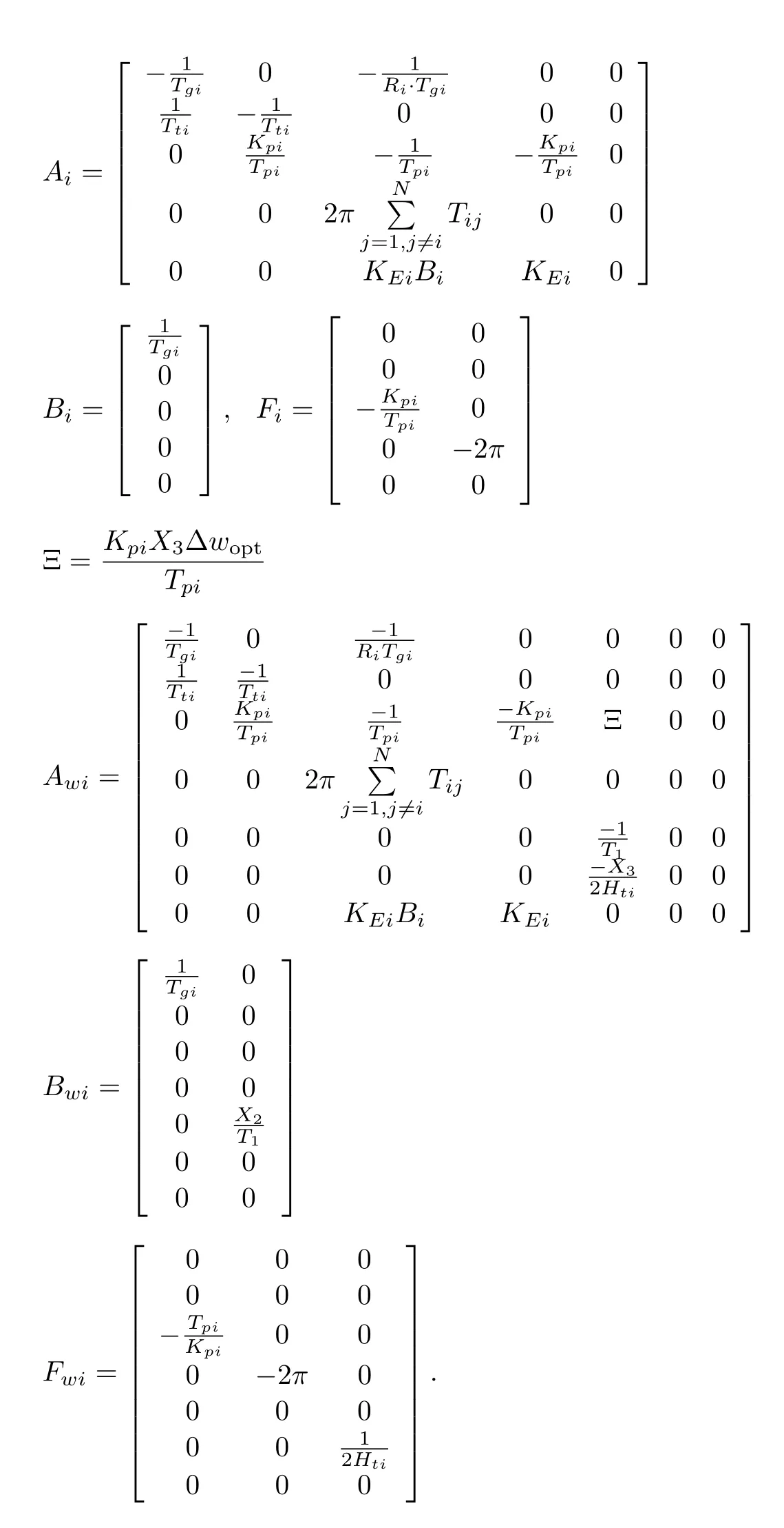
where ui(t)= ∆Pci(t)is the control input,∆Pdi(t)=[∆PLi(t)∆Vi(t)]Tis the disturbance vector.For a nominal system,the matrices Ai,Biand Fiin(5)are formulated in Appendix A.The system model(5)will be employed for the LFC design of the ith control area in the multi-area power system.

B.Simplified Wind Turbine Model

The doubly-fed induction generator(DFIG)system has been proven a proper renewable energy conversion system.A simplified frequency response model of a DFIG based wind turbine unit[10]is illustrated in Fig.2.

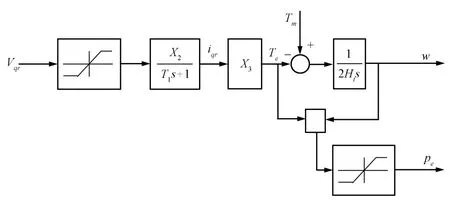
Fig.2.Simplified model of DFIG based wind turbine.

The model of the DFIG-based wind turbine unit can be described by the following equations.

where Vqr(t)and iqr(t)are the q-axis components of the rotor voltage and the rotor current,respectively.w(t)is the rotational speed,Tm(t)is the mechanical power,Htis the equivalent inertia constant,Pe(t)is the active power.Other parameters in Fig.2 are explained as X2=1/Rr,X3=Lm/Lss,T1=L0/wsRs,L0=Lrr+L2m/Lss,and Lss=Ls+Lm,Lrr=Lr+Lm,here Lmis the magnetizing inductance,Rrand Rsare the rotor and stator resistances,respectively.Lrand Lsare the rotor and stator leakage inductances,respectively.Lrrand Lssare the rotor and stator self-inductances.wsis the synchronous speed.

Linearizing the wind turbine model at a certain operating point,we can rewrite(8)as

where woptis the rotational speed at the operating point and Te(t)is the electromagnetic torque.

C.Dynamics for Wind Turbine Load Frequency Control

Equation(11)will be employed for the LFC design for wind turbines in the multi-area power system.The details about Awi,Bwiand Fwiare available in Appendix A.

Remark 1:Equation(5)presents the mathematical model for the LFC problem of the conventional generating system in control area i.Equation(5)does not consider the effects of wind turbines on the system frequency because the capacity of the wind turbine unit only shares a small proportion in the power system.On the contrary,to design a frequency controller for the wind turbine unit,some variables of the renewable power system are considered in(11).

D.Analysis About System Models

From(5)and(11),these system models can be described by a uniform expression.Without loss of generality,the expression has a form of

By considering the parameter uncertainties and the modelling errors,equation(12)can be written as

where A0,B0and F0denote the nominal constant matrices,∆A xx(t),∆B (t)and∆F∆P(t)denote the parameter uncertainties and the modeling errors.

It is noted that the above discussions just consider the uncertainties existing in the linear power system.Power systems actually cover the GRC nonlinearity.The existence of GRC has adverse effects on the system stability.Inherently,the GRC nonlinearity acts as a limiter to limit the rate of change in the power generation.Taking the turbine of generating units as an example,the limiter output remains unchanged while reaching its top or bottom.But the turbine output keeps increasing or decreasing at the extreme rate of change.This fact indicates the nonlinear power system becomes linear before the limiter output reaches its limit value.Having been triggered by the two critical points of the limiter,the turbine output is still changing but the change is at its extreme rates determined by the limiter.From Fig.1,these discussions can be formulated by

where σ(t)= ∆Xgi(t)∆Pgi(t)and δ＞ 0 is the maximum output of the GRC nonlinearity.

As far as the LFC problem of the nonlinear power system is concerned,the effect of the extreme rates only exists on the outset because∆Xgi(t)must change to make∆Pgi(t)resist the load disturbance∆PLi(t).From this perspective,the effect of the GRC nonlinearity can be treated as a kind of uncertainties.Different from the uncertainties in(13),this kind of uncertainties can attenuate their effects in the dynamic process.

From(13)and(14),the following general model can be derived for the power system.

where φ(t)denotes the uncertainties due to GRC.

From(15),the LFC design of the nonlinear power system with wind turbines can be divided into two parts.One is to design a T-SMC-based load frequency controller for the nominal system.The other is to consider how to suppress the system uncertainties.

III.CONTROL DESIGN

A.Mathematical Descriptions of the System for Terminal Sliding Mode Control

To aggregate all the uncertain terms in(15), ddd (t)is defined and formulated by

Then,the general system model(15)has a form of

Assumption 1:The uncertain term (t)in(16)satisfies ddd(t)=B0H(t)where ‖H(t)‖ ≤‖ ·‖ denotes the Euclidean norm andis constant but unknown.

According to the principle of matrix controllability decomposition,we adopt the nonsingular transformation of Z(t)=[29],[30].Then,some matrices in(17)becomes

According to(18),the following equations(19)can be derived from(17).

[zn−m+1(t) ···zn(t)]T∈ Rm.In(19),H(t)means the system uncertainties.

B.Design of Global Fast Terminal Sliding Mode Control

In[24],a kind of sliding surfaces is entitled global fast terminal sliding surface.However,this kind of surfaces in[24]is defined in the scalar form such that it cannot be directly employed for the LFC problem of renewable power systems.To develop a global fast terminal sliding surface for the LFC problem,the general sliding surface vector(20)is extended for multi-variable systems[31].The extended global fast terminal sliding surface vector for the nominal part of(19)is formulated by

where (t)∈ Rm×1,C1∈ Rm×(n−m),C2∈ Rm×m,C3∈ Rm×(n−m).Both p and q are positive and odd numbers,andis a vector,defined byC2is non-singular to guarantee C2B2invertible.Matrices C2and C3are selected to satisfy the following equations.

In(21)and(22),αi＞ 0,βi＞ 0,i=1,2,...,n−m.When A12is row full rank,the right inverse of A12denoted byexists and has a form of

From(21)and(22),C1and C3can be selected as follows.

Differentiating s(t)in(20)with respect to time t and substituting(19)into the derivative of(20),we get(26).

When the system trajectory enters the sliding mode stage and keeps on the sliding surface, sss˙ (t)=Omexists,here Om∈Rm×mis an m-dimensional vector of zeros.Without regard to uncertainties,the equivalent control law of the T-SMC system can be deduced from(t)=Om,determined by

Consider(19)and define the global fast terminal sliding surface(21).Then,the final T-SMC law[31]can be formulated by

where η ＞ 0.

Remark 2:Since the T-SMC law(28)contains¯h0,the value of¯h0must be known in advance to guarantee the system stability.In other words,the control law(28)is available for the LFC problem under the condition that the uncertainties are with a known boundary.Unfortunately,the boundary value is rather difficult to know in practice.As displayed in Assumption 1,the LFC system is designed under the assumption that the uncertainties have an unknown boundary.Consequently,it is necessary to consider how to deal with the issue.

C.Design of RBF Neural Networks

To fill the gap between the system stability and the boundary value of uncertainties,RBF NNs are employed because such a kind of neural networks owns the ability to approximate complex nonlinear mapping directly from input-output data with a simple topological structure.RBF NNs are a kind of three-layer feed-forward networks,where the mapping from the input layer to the output layer is inherently nonlinear but the mapping from the hidden layer to the output layer is linear.

Fig.3 displays the designed RBF NNs.Concerning the LFC problem,each element of the state vector xxx(t)in(17)is employed as an input element,where γ=1,...,n.Accordingly,the network output y is defined as the estimated value of the system uncertainties.In other words,the designed RBF NNs have n inputs and 1 output.Illustrated in Fig.3,there are l neurons in the hidden layer.

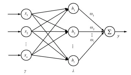
Fig.3.Structure of RBF NNs.

From Fig.3,the output of the RBF NNs is determined byThen,the network output can be calculated by

where λ =1,2,...,l,cλ∈ Rnis the center vector of the λth Gaussian function,bλis a scalar,indicating the width of the λth Gaussian function.Both cλand bλare predefined parameters.

Adopting the RBF approximation technology,the control law(28)can be rearranged by

Remark 3:The term h(t)depicts the system uncertainties.Not only is h(t)hard to be formulated,but also its boundary value is difficult to be obtained.To guarantee the network output can match the change of uncertainties,each element of the weight vector ω has to be renewed by an update law.It is necessary to obtain the update law of the weight vector.On the other hand,the update law makes a difference to the system stability.Consequently,this topic will be investigated in the sense of Lyapunov.

D.Stability Analysis

Assumption 2:There exists an optimal weight vector ω∗such thatsatisfies

Assumption 3:The boundary valueminus the Euclidean norm of the system uncertainties satisfies

Theorem 1:Take Assumptions 1−3 into account,consider the system model(17),define the global fast terminal sliding surface(20),and adopt the control law(31).Then,the T-SMC-based LFC system is of asymptotic stability if and only if the update law of the network weight vector has a form of

where ξ is a constant and satisfies

Proof:Consider the candidate Lyapunov function

Differentiate V with respect to time t in(36).The derivative of V can be formulated by

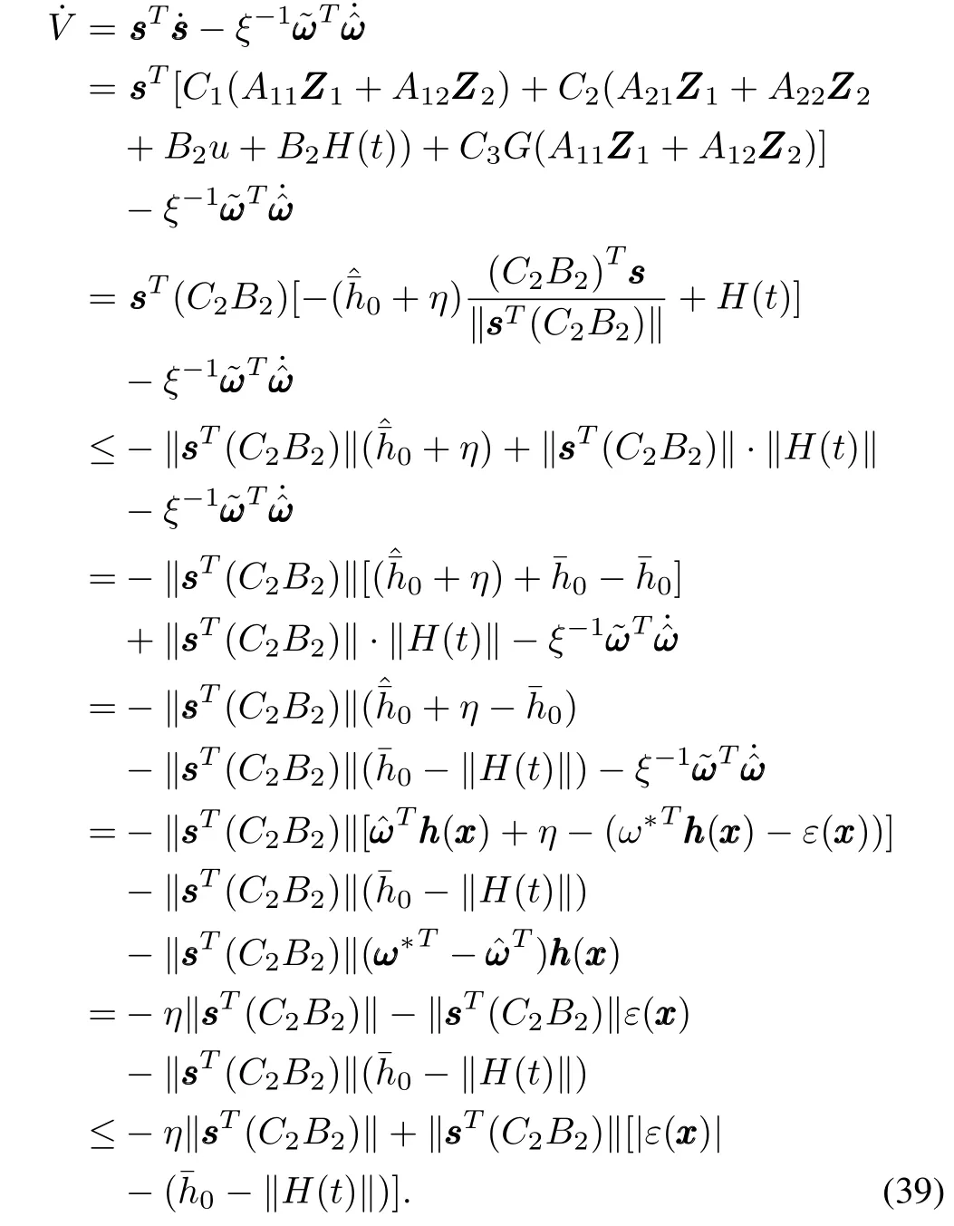
Taking Assumptions 2 and 3 into account,we can conclude that the inequalityexists.Then,(39)becomes

From(36)and(40),we have V≥0 and˙V≤0.Further,(41)can be deduced from(36).

Integrating both sides in(42)yields

The time τ can be calculated by

In the sense of Lyapunov,V will reach zero from the state of V0in the finite time τ.Meantime,the global fast terminal sliding surface sss (t)reaches zero.This also indicates that the state variables of the proposed power system will enter the sliding mode stage in a finite time.

On the sliding surface,there is

Since C2is nonsingular,(46)can be obtained

Substituting(46)into(19)yields

By selecting C1,C2and C3in(24)and(25),the derivative of ZZZ1can have the form of

From(48),each element in bothwill rapidly converge to zero in a finite time.Further, ZZZ2is the linear combination ofin(46)such that each element in ZZZ2will converge to zero in a finite time as well as ZZZ1.Since ZZZ is defined by the form of,each element in ZZZ and x will definitely converge to zero in a finite time.

Consequently,the closed-loop LFC control system is asymptotically stable in the sense of Lyapunov.In this regard,not only can the designed update law(34)guarantee the convergence of the RBF NNs,but also the whole LFC system can earn the asymptotic stability by such a control scheme.■

Remark 4:From(19), uuueqin(27)can be rewritten as

Remark 5:An inherent drawback of the sliding mode control technique is chattering[14].To reduce the chattering,the smooth processing should be adopted for the relay characteristics in(31)[32].The amendment has the form of

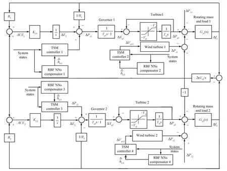
Fig.4.Block diagram of the considered two-area power system.

where δ is a small positive constant.

Remark 6:According to the designed control scheme,the GRC nonlinearity is transformed into a part of system uncertainties.The RBF NNs can be treated as a compensator to approximate and compensate the entire system uncertainties.The compensator and the controller cooperate to overcome the LFC problem for the nonlinear power system with wind turbines.

Remark 7:The generating unit with GRC in Fig.1 and the wind turbine in Fig.2 simultaneously exist in a control area.Both of them can affect the frequency of the considered control area.Hence,two load frequency controllers and their compensators in one control area should be designed to achieve the LFC task according to(5)and(11),respectively.

IV.SIMULATION RESULTS

Consider the LFC problem of renewable power systems.An interconnected power system with wind turbines is employed to illustrate the effectiveness and feasibility of the proposed TSMC scheme.The power system is composed of two control areas.Each control area has an aggregated generating unit with GRC in Fig.1 and an aggregated wind turbine unit in Fig.2.As mentioned above,the generating unit and the wind turbine mean all generator units and all wind turbines in the control area are aggregated together.The proposed control scheme will be carried out by the LFC solution of such a nonlinear interconnected power system,where the system schematic is illustrated in Fig.4.

Some parameters and data from the interconnected power system[10]are listed in Table I.The power system consists of two 800MVA-scale control areas.Wind turbine parameters[10]are listed in Table II,where the wind speed vwind=11m/s,the rotational speed vr=1.17m/s,Xmis the magnetizing reactance,(wr)base= 1.15rad/s.The wind turbine parameters originate from the 247MW operating point,where the turbine power composed of 200 units of 2MW wind turbines is 400MVA-scale.The gains of the two additional states in the two control areas are selected as KE1=KE2=1.According to the listed parameters,the nominal models of the interconnected power system in Fig.4 can be obtained.Subsequently,the models can be employed for the LFC design.

As mentioned above,some controller parameters are pre-defined.Concerning the T-SMC-based controllers in Areas 1 and 2,thetransformation matrices Tr(r=1,...,4)for each controller design are specified by

TABLE IPARAMETERS AND DATA OF TWO CONTROL AREAS

TABLE IIWIND TURBINE PARAMETERS AT 247MW OPERATING POINT(p.u)

For Controllers 1 and 3,C1=C3=[1 2 3 4],C2=1.For the other two controllers in Fig.4,their parameters are determined by

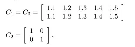
Other controller parameters are determined by p=9,q=7,η=0.1 and δ=0.04.

Concerning the designed RBF NNs,some network parameters should also be set up.For RBF NNs 1 and 3,place 6 neurons in their hidden layers,select the initial weights between the hidden and output layers as[0.1 0.1 0.1 0.1 0.1 0.1]T,and determine the widths of the Gaussian function vector as[0.2 0.2 0.2 0.2 0.2 0.2]T.For RBF NNs 2 and 4,place 8 neurons in their hidden layers,select their initial weights as[0.1 0.1 0.1 0.1 0.1 0.1 0.1 0.1]Tand determine the widths of the Gaussian function vectors as[0.2 0.2 0.2 0.2 0.2 0.2 0.2 0.2]T.For the four RBF NNs,all their centers take random numbers between−1 and 1.Other parameters for the four RBF NNs are defined by ε0=0.002 and ε1=0.001.

To show the performance of the presented method,two step load disturbances PL1=PL2=1%are simultaneously applied to the interconnected power system at t= 5s.Fig.5 illustrates the comparisons of frequency deviations,area control errors and deviations of the tie-line active power,where the blue solid lines mean the LFC system has RBF NNs and the red dashed lines mean the LFC system has no RBF NNs.Under the condition of no RBF NNs,the boundary of system uncertainties is assumed to be known such that the control law(50)is directly adopted.The other controller parameters are kept unchanged.

From Fig.5,∆f,ACE and∆Ptieare damped to zero after disturbances with small oscillations in a finite time.Without doubt,the system state changes of the LFC system with RBF NNs are a little smoother and the settling times are slightly shorter.Anyway,the control performances of the two control methods can just make a little difference on the aspect of these state variables.

Fig.6 illustrates the control inputs in the two control areas,where the red solid lines indicates the LFC system without RBF NNs and the blue solid lines indicates the LFC system with RBF NNs.To guarantee the system stability,the LFC system without RBF NNs needs to predefine a large¯h0since the LFC system suffers from the severe chattering phenomenon.On the other hand,the LFC system with RBF NNs can adaptively approximate the boundary of the system uncertainties such that the curves of the control inputs are much smoother.In this sense,the designed RBF NNs contribute to a significant reduction of the chattering phenomenon.Further,the outputs of the designed RBF NNs are illustrated in Fig.7.As proven in Theorem 1,not only can the update law(34)make the networks convergent,but also the LFC control system possesses the asymptotic stability.

To demonstrate the control performance of the presented control scheme,the comparisons between the presented scheme and the SMC method with RBF NNs are shown in Fig.8.In Fig.8,the RBF NNs parameters in the two LFC control systems make no difference.The control performance is just decided by the two control methods.

Compared with the results of the SMC method with RBF NNs,the performance of the presented control scheme is better without doubt.Especially,the overshoot of the presented method in Fig.8 is zero which shows that the presented control scheme is more robust against load disturbances in power systems with wind turbines.

V.CONCLUSIONS

This article has addressed the LFC problem for renewable power systems in the presence of GRC.The control scheme is designed by means of T-SMC.To suppress the uncertainties of the LFC problem,RBF NNs are adopted.The theoretical analysis in the sense of Lyapunov proves that the T-SMC-based LFC system is asymptotically stable.The presented control scheme has solved the LFC problem of an interconnected renewable power system composed of two control areas.Some numerical simulation results have demonstrated the performance of the presented method against uncertainties of nonlinear power systems with renewable sources.

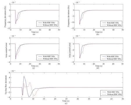
Fig.5.Simulation results of the interconnected power system with and without RBF NNs.(a)Frequency deviation∆f1in Area 1.(b)Frequency deviation∆f2in Area 2.(c)Area control error ACE1in Area 1.(d)Area control error ACE2in Area 2.(e)Deviation of tie-line active power∆Ptie.

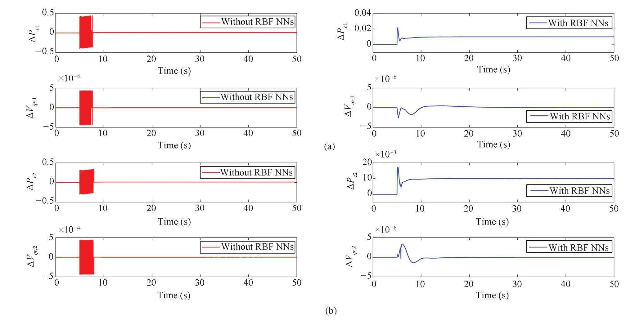
Fig.6.Simulation results of control inputs.(a)Control inputs in Area 1.(b)Control inputs in Area 2.

Fig.7.Simulation results of RBF NN outputs.(a)RBF NN outputs in Area 1.(b)RBF NN outputs in Area 2.

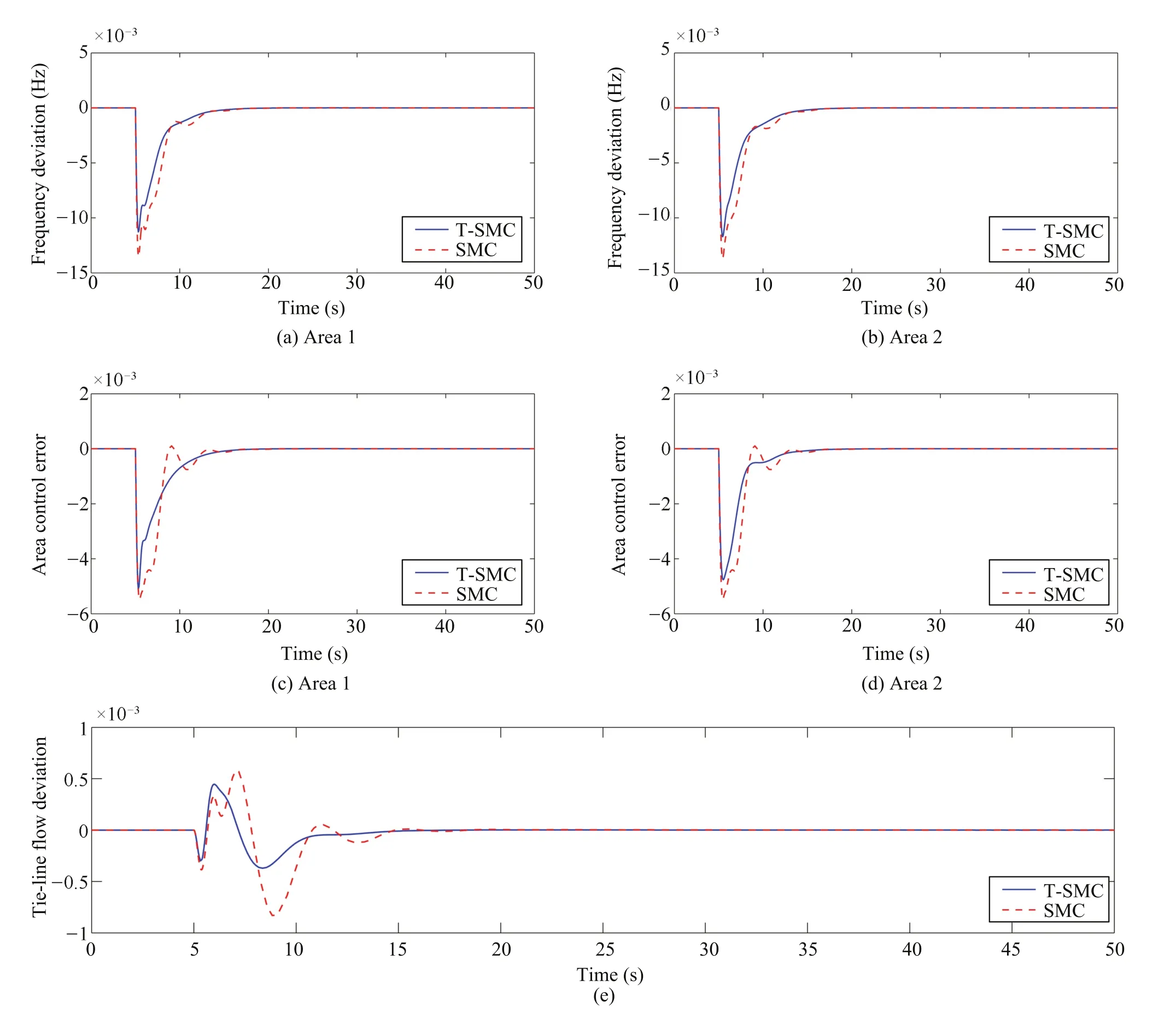
Fig.8.Comparisons between T-SMC with RBF NNs and SMC with RBF NNs.(a)Frequency deviation∆f1.(b)Frequency deviation∆f2.(c)Area control error ACE1.(d)Area control error ACE2.(e)Deviation of tie-line active power∆Ptie.

APPENDIX PARAMETER MATRICES