Design of a spatial sampling scheme considering the spatialautocorrelation of crop acreage included in the sampling units

WANG Di, ZHOU Qing-bo, YANG Peng, CHEN Zhong-xin

Key Laboratory of Agricultural Remote Sensing, Ministry of Agriculture/Institute of Agricultural Resources and Regional Planning,Chinese Academy of Agricultural Sciences, Beijing 100081, P.R.China

Abstract Information on crop acreage is important for formulating national food polices and economic planning. Spatial sampling,a combination of traditional sampling methods and remote sensing and geographic information system (GIS) technology,provides an efficient way to estimate crop acreage at the regional scale. Traditional sampling methods require that the sampling units should be independent of each other, but in practice there is often spatialautocorrelation among crop acreage contained in the sampling units. In this study, using Dehui County in Jilin Province, China, as the study area, we used a thematic crop map derived from Systeme Probatoire d’Observation de la Terre (SPOT-5) imagery, cultivated land plots and digital elevation model data to explore the spatialautocorrelation characteristics among maize and rice acreage included in sampling units of different sizes, and analyzed the effects of different stratification criteria on the levelof spatialautocorrelation of the two crop acreages within the sampling units. Moran’s I, a global spatialautocorrelation index, was used to evaluate the spatialautocorrelation among the two crop acreages in this study. The results showed that although the spatialautocorrelation levelamong maize and rice acreages within the sampling units generally decreased with increasing sampling unit size, there was stilla significant spatialautocorrelation among the two crop acreages included in the sampling units (Moran’s I varied from 0.49 to 0.89), irrespective of the sampling unit size. When the sampling unit size was less than 3 000 m, the stratification design that used crop planting intensity (CPI) as the stratification criterion, with a stratum number of 5 and a stratum intervalof 20% decreased the spatialautocorrelation level to almost zero for the maize and rice area included in sampling units within each stratum. Therefore, the traditional sampling methods can be used to estimate the two crop acreages. Compared with CPI, there was stilla strong spatial correlation among the two crop acreages included in the sampling units belonging to each stratum when cultivated land fragmentation and ground slope were used as stratification criterion. As far as the selection of stratification criteria and sampling unit size is concerned, this study provides a basis for formulating a reasonable spatial sampling scheme to estimate crop acreage.

Keywords: crop acreage, spatialautocorrelation, sampling unit, planting intensity, cultivated land fragmentation, ground slope

1. Introduction

Information on crop acreage and yield is a crucial element in formulating national food policies and economic planning(Carfagna and Gallego 2005). Timely availability of crop area information plays a very important role in forecasting crop production, formulating agricultural policies and ensuring national food security (Reynolds et al. 2000; Tao et al. 2005; Song et al. 2017). For a long time, crop acreage data have been routinely surveyed and updated by China’s statistical department mainly using the traditional multilevel list sampling method, in which sample counties are drawn from the provinces, and then sample villages are drawn from sampled counties, andfinally sample households are drawn from the sampled villages (NBSC 2002). However,the operational problems facing the list sampling survey include: slow update of the sampling frame, insufficient use of spatial information technology during the survey, and human in fluence on the survey results. Consequently, the accuracy and timeliness of the crop acreage survey remain poor. With the development of earth observation technology,satellite-based remotely sensed data have the unique advantage of providing continuous spatialand temporal information on crop cultivation and growth at various regional scales, owing to its wide real-time coverage. Therefore, it has often been combined with traditional sampling methods,to estimate the crop acreage over a large region.

Compared with the traditional list sampling survey,spatial sampling transforms the investigation object from a farmer household into a cultivated land plot. It can,therefore, achieve more accurate crop acreage information.Moreover, using satellite-based remotely sensed data increases the timeliness of crop area surveys in conjunction with spatial sampling. The use of remotely sensed data in sampling surveys for crop acreage estimation began in the early 1970s. The Large Area Crop Inventory Experiment(LACIE), conducted jointly, in 1974, by the United States Department of Agriculture (USDA) and the Nationalaeronautics and Space Administration (NASA) is a typical example. Satellite images were used to derive a thematic map of wheat distribution, and this was the basis for a stratified sampling scheme (Macdonald and Hall 1980).More recent projects include the Agriculture and Resource Inventory Surveys through Aerospace Remote Sensing(AGRISARS) (Benedetti et al. 2010) and the Monitoring Agriculture with Remote Sensing (MARS) Project (now named CROP4CAST) sponsored by the European Union.The latter used stratified sampling to monitor and estimate the acreage of 17 crops. In that project, satellite images were employed to formulate a stratification scheme and to measure crop acreages within the sampled units (Gallego 2004; Carfagna and Gallego 2005). Previous studies on crop acreage estimation using the spatial sampling method have focused mainly on how to improve the survey accuracy and timeliness, and decrease the survey cost and workload,by combining traditional sampling methods with remotely sensed data. In these studies, simple random sampling,systematic sampling, stratified sampling and multistage sampling methods have often been used, and the crops involved included wheat, rice, maize and cotton.

The deficiencies of the list sampling survey can thus be effectively addressed by combining traditional sampling methods and remotely sensed data. However, traditional sampling is based on classical statistical theory, which is appropriate when researching changes in purely random variables. These methods treat the sampling units, when used to estimate population parameters, as independent.In practice, the in fluence of natural conditions (climate, soil type, topography, and landforms), socioeconomic factors,and crop distributions mean the sampling units, at the regional scale, are not independent and exhibit a degree of spatialautocorrelation. Traditional sampling methods cannot address this spatialautocorrelation. Many previous studies have indicated that the spatialautocorrelation of such key variables should be considered in spatial sampling(Overmars et al. 2003; Gertner et al. 2007; Buarque et al.2010; Le Rest et al. 2013; Holmberg and Lundevaller 2015).Neglect of spatialautocorrelation may lead to overestimation of variance and require sample size, and possibly a false conclusion (Lichstein et al. 2002; Betts et al. 2006; Frutos et al. 2007; Hoeting 2009; Kulkarni and Mohanty 2012;Melecky 2015).

Spatialautocorrelation refers to correlations that exist between the observed values of a single attribute/variable at different locations across an area, and is a measure of the degree of spatial clustering of the attribute (Cliff and Ord 1981; Griffith 1988). Spatialautocorrelation is common within geographic data and is found in diverse spatial variables, contexts and structures (Legendre and Legendre 1998; Keitt et al. 2002). Since Tobler (1970) put forward his First Law of Geography, studies on spatialautocorrelation among geographicalattributes have been undertaken by many researchers (Cliff and Ord 1981; Anselin 1988;Goodchild et al. 1993; Fisher et al. 1996; Haining 2003).The levelof spatialautocorrelation can be estimated using a globalor a local indicator. A global indicator is used to detect spatial clustering across a whole study territory, with the area’s spatialautocorrelation represented by a single value. To date, Moran’s I remains the most commonly used statistical indicator for global spatialautocorrelation(Holmberg and Lundevaller 2015; Melecky 2015). Using Moran’s I as the statistical indicator, the referenced studies have demonstrated the existence of spatialautocorrelation within various geographical variables, explored the characteristics and variations in spatialautocorrelation, and analyzed its in fluence on required sample size, population extrapolation and estimated error in a sampling survey.

Although studies on spatialautocorrelation among sampling units have been conducted for more than a decade,these studies have focused mainly on animal conservation(Frutos et al. 2007; Le Rest et al. 2013),fishery resources(Jardim and Ribeiro 2007), forest community structures(Gilbert and Lowell 1997) and land use (Overmars et al.2003). There are no reports on the spatialautocorrelation of crop acreage including the sampling units, moreover, factors affecting the spatialautocorrelation of crop acreage have not previously analyzed. This complicates the application of spatial sampling in crop acreage monitoring in conjunction with remote sensing. The main objectives of this study were to: (i) investigate the spatialautocorrelation among crop acreage included in sampling units of different sizes;(ii) analyze the effects of different stratification criteria on the spatialautocorrelation levelof crop acreage within the sampling units; (iii) suggest reasonable stratification criteria and sampling unit sizes for spatial sampling scheme to estimate crop acreage.

2. Materials and methods

2.1. Analysis process

The analysis process consisted of seven steps. the first step was the preparation of the basic data used to formulate the spatial sampling scheme for crop acreage estimation. Step two was the selection of the spatialautocorrelation index.The global Moran’s I was used to evaluate the degree of spatialautocorrelation of crop acreage within the sampling units. The third step was the design of the sampling unit sizes and the construction of sampling frames with different unit sizes. Step four was the analysis of spatialautocorrelation of crop acreage within the different sized sampling units.Thefifth step was the formulation of the stratified sampling strategy, including the design of the stratification criteria,strata number and intervals. Step six was the spatialautocorrelation analysis of crop acreage in the sampling units belonging to different strata. The last step was the optimization of the stratification criteria and sampling unit size in the spatial sampling scheme for crop acreage estimation.Fig. 1 shows the overall flowchart for this study.

2.2. Study area

Dehui County in Jilin Provine, China, was chosen as the study area because of the availability of high-quality crop distribution, cultivated land and digital elevation model (DEM)data covering the whole region, at similar times. Moreover,the topography and spatial distribution of crops that are found in Dehui County are representative of a wider area and, therefore, indicative for analysis of spatial correlation of variables used in defining sampling units for crop acreage estimation. Dehui County is located in the north central part of Jilin Province, Northeast China (44°02´-44°53´N latitude,125°14´-126°24´E longitude), with a total land area of 3 460 km2(Fig. 2). It includes a total cultivated land area of 2 540 km2. It has a sub-humid continental monsoon climate with four distinct seasons. The annualaverage temperature is 4.4°C, the average annual hours of sunshine are 2 695.2 h,the average annual frost-free period is 139 days, and the average annual precipitation is 520 mm. Within the agricultural sector, priority is given to food crops, while cash crops are complementary. Food crops include maize, rice,soybean and sorghum. Maize and rice are two particularly important food crops in Dehui County.

2.3. Data preparation

First, the administrative boundary (from 1:10 000 mapping)of Dehui County was acquired to define the extent of the sampling survey for maize and rice acreage estimation and to help construct the spatial sampling frame. Second,cultivated land plots covering the study area were extracted from the Second National Land Survey,finished by China in 2009, and used to calculate plot fragmentation. Third,maize and rice growing areas were extracted from three Systeme Probatoire d’Observation de la Terre (SPOT-5)images (track numbers: 296-260, 296-261 and 297-260,date: 08-01-2009, spatial resolution: 10 m), to determine the planting intensity within each sampling unit. Finally,for the study area, we downloaded the freely available ASTER Global Digital Elevation Model (GDEM) (version 2) with a resolution of 30 m in GeoTIFfformat, and from this computed the ground slope within each sampling unit.Figs. 3 and 4 show the spatial distributions of cultivated land plots, and maize and rice distributions. Fig. 5 shows the land elevations (from the GDEM).

2.4. Selection of spatialautocorrelation index

The global spatialautocorrelation index (Moran’s I)quantitatively describes the spatial dependence existing between variable values, and has been widely used to evaluate the spatialautocorrelation of variables of interest.Compared with Geary’s C, the distribution characteristics of Moran’s I are easier to depict with an estimator (Cliff and Ord 1981). Hence, we selected this method to evaluate the spatialautocorrelation of the sampling units. Moran’s I ranges from −1 to +1. The closer a value of Moran’s I is to+1, the stronger is the positive spatialautocorrelation of the variable being analyzed among the sample plots. When the value of Moran’s I is equal to or approximately zero, there is no spatialautocorrelation and the values of the analyzed variable in the sampling units are random (not spatially related). For maize, the global Moran’s I as calculated by Cliff and Ord (1981) is:

Fig. 1 The overall flowchart of this study.

Where, I is the global spatialautocorrelation index; n is the number of sampling units; yiis the maize planting area in the ith sampling unit; yjis the maize planting area in the jth sampling unit; y is the average value of maize planting area in all sampling units; and Wijis the spatialadjacency between sampling units i and j. The spatialadjacency matrix was calculated using ArcGIS Software, and its type was Contiguity-Edges-Corners, which means the sampling units that share a boundary or node will in fluence the computation of the target unit. The same equation was applied to rice area and the other analyzed variables.

The significance of Moran’s I is tested based on the Z-score as given by eqs. (2)-(6). The Z-score was also calculated using ArcGIS Software.

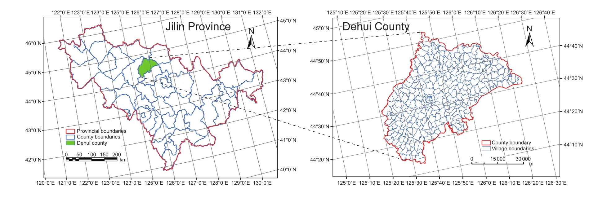
Fig. 2 Location of the study area in Jilin Province, Northeast China.

Where, wi.is the sum of all elements belonging to the ith line in the spatialadjacency matrix wij; w.jis the sum of all elements belonging to the jth row in the spatialadjacency matrix wij.

2.5. Design of sampling unit sizes

We chose a square grid as the shape of the sampling units to facilitate the calculation of the adjacency matrix and hence Moran’s I. To determine the in fluence of sampling unit size on the spatialautocorrelation of the variables, we formulated 25 levels of sampling unit size. Using a size intervalof 200 m,the 25 sampling unit sizes were 200 m×200 m, 400 m×400 m, …, 5 000 m×5 000 m. The study area was then divided into these square grids to construct 25 sampling frames. When a square grid crossed or was within the administrative boundary of the study area, it belonged to the sampling frame.

2.6. Stratification on crop planting intensity within sampling units

Crop planting intensity (CPI) is the proportion of a sampling unit being cropped. In this study, we calculated the CPI of each crop, for each sampling unit, by independently overlaying the maize and rice spatial distribution data on the sampling frame. Comprehensively considering the decrease of variance within the strata, the feasibility of sample selection and the computation of spatialautocorrelation among crop areas in the sampling units, the CPI values in all sampling units were then divided intofive strata: (1)0.01-20%; (2) 20-40%; (3) 40-60%; (4) 60-80%; and(5) 80-100%. Accordingly, all sampling units were also divided intofive strata based on the stratification of their CPI value. The spatialautocorrelation levelamong crop acreages included in the sampling units of each stratum was determined using the global Moran’s I. Using seven sampling unit sizes (200 m×200 m, 500 m×500 m, 1 000 m×1 000 m, 2 000 m×2 000 m, 3 000 m×3 000 m, 4 000 m×4 000 m, 5 000 m×5 000 m), as examples, we computed the spatialautocorrelation levelamong crop acreages included in the sampling units of each stratum at each sampling unit size. Although the size of 500 m×500 m was not listed above,this is widely used tofield survey crop acreage in China, so we added this size between 200 m×200 m and 1 000 m×1 000 m as a representative example. Using the sampling unit size of 1 000 m×1 000 m as an example, Fig. 6 shows the spatial distribution of the sampling units stratified by the maize and rice CPI values.

2.7. Stratification on cultivated land fragmentation within the sampling units

Cultivated land fragmentation is often defined as the division of a cropland type into smaller parcels (Nagendra et al.2006). The stratification on cultivated land fragmentation may have a potential in fluence on the spatialautocorrelation levelof crop area in the sampling units, as crops are generally planted on cultivated land. We designed a fragmentation index (FRG) to quantitatively describe the degree of cultivated land fragmentation within each sampling unit. The FRG is calculated using eq. (7).

Where, FRGiis the cultivated land fragmentation within the ith sampling unit; Niis the number of cultivated land plots within the ith sampling unit; Aiis the totalarea (in ha)of all cultivated land plots within the ith sampling unit. We sorted the FRG of all sampling units into ascending order and divided them intofive strata based on their rank, keeping the number of sampling units within each stratum almost equal. the five strata offRG were: (1) 0.05-0.16; (2)0.16-0.20; (3) 0.20-0.26; (4) 0.26-0.35; and (5) 0.35-9.20.Accordingly, all sampling units were also divided intofive strata based on the stratification of their FRG. The spatialautocorrelation levelamong crop acreages included in the sampling units of each stratum was also determined using the global Moran’s I index. As with the CPI, we computed the spatialautocorrelation levelamong crop acreages included in the sampling units of each stratum at each of seven sampling unit sizes. Using the sampling unit size of 1 000 m×1 000 m as an example, Fig. 7 shows the spatial distribution of the sampling units stratified by their FRG.

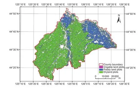
Fig. 3 Spatial distribution of cultivated land in Dehui County,Jilin Province, China.

Fig. 4 Spatial distribution of maize and rice in Dehui County,Jilin Province, China.

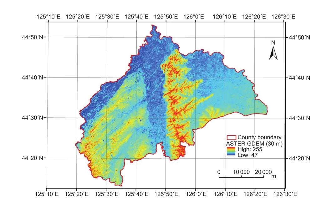
Fig. 5 Land elevation in Dehui County, Jilin Province, China.

Fig. 6 Spatial distribution of sampling units stratified by the crop planting intensity of maize and rice on a 1 000 m×1 000 m grid.

2.8. Stratification on the average ground slope of the sampling units

The ASTER GDEM data were processed through tessellation, projection conversion and slope calculation,and the average ground slope within each sampling unit was then determined. The average values of ground slope were sorted from the smallest to largest, and then divided intofive strata based on the rank: (1) 0.34-0.87%;(2) 0.87-1.01%; (3) 1.01-1.23%; (4) 1.23-1.82%; and (5)1.82-11.64%. All sampling units were also divided intofive strata based on the stratification of ground slope. As with the CPI, seven sampling unit sizes were used, and the spatialautocorrelation levelamong crop acreages included in the sampling units of each stratum at each sampling unit size was computed. Using the sampling unit size of 1 000 m×1 000 m as an example, Fig. 8 shows the spatial distribution of the sampling units stratified by their average ground slope.

Fig. 7 Spatial distribution of the sampling units stratified by their fragmentation index (FRG) on a 1 000 m×1 000 m grid.

3. Results

3.1. Spatialautocorrelation and its significance at different sampling unit sizes

To demonstrate that there is spatialautocorrelation within the sampling units, Fig. 9 shows the values of the Moran’s I and Z-score for maize and rice areas, as shown in Fig. 3,at 25 different sampling unit sizes. For both maize and rice, the Moran’s I value decreased as the sampling unit size increased, while the Z-score value increased with the sampling unit size. Furthermore, when the sampling unit size was less than 1 000 m, Moran’s I value decreased rapidly, varying from 0.89 to 0.65. However, when the sampling unit size was greater than 1 000 m, the decrease of Moran’s I value slowed down until it became stable, and varied from 0.65 to 0.49. This indicated that 1 000 m was the in fl ection point where the curve of the Moran’s I value changed with the sampling unit size. The Moran’s I values for maize and rice for the 25 sampling unit sizes ranged from 0.49 to 0.89. The corresponding Z-score values were all greater than 300, which indicated very significant spatialautocorrelation of maize and rice acreage between the sampling units. The values of Moran’s I and Z-scores for rice were greater than those for maize, regardless of the sampling unit size. The reason was that the growing region of rice was more concentrated than that of maize,in this study area.

3.2. lnfluence of CPl stratification on spatialautocorrelation among crop acreages in the sampling units

Fig. 8 Spatial distribution of the sampling units stratified by their average ground slope on a 1 000 m×1 000 m grid.

To illustrate the spatialautocorrelation of CPI between sampling units, Fig. 10 shows the changes of Moran’s I values for the maize and rice sampling units for the five planting intensity levels. When the sampling unit size was less than or equal to 3 000 m, the change ranges and absolute values of Moran’s I were both very small.However, when the sampling unit size was greater than 3 000 m, the amplitudes and absolute values of Moran’s I significantly increased for both maize and rice. In addition,when the sampling unit size was less than 3 000 m, the Moran’s I values of the planting intensity class variable for both crops were less than 0.2, which denoted very little spatialautocorrelation of the CPI strata for either maize or rice sampling units. Thus, for this variable, conventional sampling methods can be used to select the sample units,and then extrapolate the results to population values. In addition, it can be also seen that the changes of Moran’s I values were relatively regular for maize and rice, when the sampling unit size was less than 3 000 m; however,the changes of the Moran’s I values become very irregular,when the sampling unit size was greater than 3 000 m. This indicated that Moran’s I can be simulated when sampling units were limited within 3 000 m.

3.3. lnfluence of cultivated land fragmentation stratification on spatial autocorrelation among crop acreages in the sampling units

Fig. 9 Moran’s I and Z-scores for different sampling unit sizes.

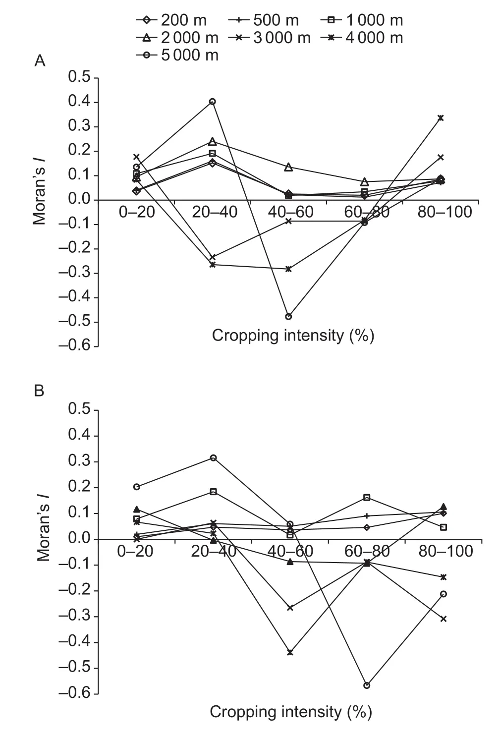
Fig. 10 Moran’s I values for different cropping intensities in maize (A) and rice (B) sampling units. Seven solid lines denote different sampling unit sizes.

Fig. 11 shows the changes in Moran’s I values of maize and rice sampling units forfive levels offRG, respectively. The profile of Moran’s I value could be classified into two types:the first was the profile when the sampling unit size was 4 000 and 5 000 m, and the second was the profile when the sampling units were sizes of 200, 500, 1 000, 2 000 and 3 000 m. For the first profile, when the sampling unit size was greater than 3 000 m, the Moran’s I values fluctuated irregularly; however, the Moran’s I values in the second profile, where the corresponding sampling unit sizes were all less than or equal to 3 000 m, decreased steadily as the cultivated land fragmentation increased. This was because the higher the cultivated land fragmentation of the sampling unit, the more scattered were the cultivated land plots within the unit. Therefore, the degree of crop clustering of planting became lower, reducing spatialautocorrelation. Three kilometers may be a threshold size for the efficient estimation of the spatialautocorrelation between the sampling units for crop acreage estimation. In addition, when the sampling unit size was less than 3 000 m, although the Moran’s I value of maize and rice distribution decreased as the levelof cultivated land fragmentation increased, this value still ranged from approximately 0.9 to 0.5 and FRG remained quite strongly autocorrelated. This implied that the levelof cultivated land fragmentation, at all sampling sizes, had little effect on decreasing the degree of spatialautocorrelation.

3.4. lnfluence of ground slope stratification on spatialautocorrelation among crops acreage in the sampling units

Fig. 11 Moran’s I values for cultivated land fragmentation in maize (A) and rice (B) sampling units. Seven solid lines denote different sampling unit sizes.

To explore the spatialautocorrelation of ground slope,Fig. 12 shows the Moran’s I values forfive ground slope levels in maize and rice sampling units. For maize, when the sampling unit size was less than or equal to 1 000 m, the Moran’s I value was the highest in the 0.87-1.01% class,and less at lower or higher slope values. This was because the average value of the ground slope of all sampling units with maize was 0.99%, and this value just fell within the range belonging to the second class of the ground slope.The implication was that most sampling units with maize were contained in the second class of ground slope, and therefore, there was a strong spatialautocorrelation within this slope class. For rice, the Moran’s I was lower when the average ground slope of sampling units was higher, except when the sampling size was greater than or equal to 3 000 m.This indicated that the spatialautocorrelation of the sampling units can be estimated, when the sampling unit size is greater than or equal to 3 000 m. Moreover, when the ground slope was in the minimum class, the Moran’s I value was the highest. Rice is often planted in low and flat areas because of its need for water. Therefore, the smaller the ground slope, the more intensive the rice planting and,consequently, the greater the Moran’s I value.

4. Discussion

Fig. 12 Moran’s I values for different ground slopes in maize(A) and rice (B) sampling units. Seven lines denote different sampling unit sizes.

Crop acreage information is the crucial basis for formulating national food policies and economic planning. Spatial sampling, the combination of traditional sampling methods and remote sensing and geographic information system technology, provides an effective measure for crop acreage estimation at the regional scale. Traditional sampling requires that the sampling units should be independent each other, but in practice there is often spatialautocorrelation among crop areas included in the sampling units. To improve the rationality of the spatial sampling scheme for crop acreage estimation, this study investigated the spatialautocorrelation among crop acreage included in sampling units of different sizes, and analyzed the effects of different stratification criteria on the levelof spatialautocorrelation of crop acreage within the sampling units, based on crop thematic mapping, cultivated land plots and DEM data covering the whole study area. The results indicated that there was strong spatialautocorrelation among maize and rice acreage included in the sampling units, no matter what the sampling unit size is. When the sampling unit size was less than 3 000 m, the stratification design with CPI was selected as the stratification criterion, the stratum number was 5 and the stratum interval was 20%, we found that the spatialautocorrelation level could be reduced almost to zero. Consequently, traditional sampling methods can be reasonably used to estimate crop area. Overall, from the perspective of the reasonable selection of sampling unit size and stratification criteria, this study provides an important basis for formulating an effective spatial sampling scheme for crop acreage estimation, based on the analysis of spatialautocorrelation of crop area contained in the sampling units.

Geographic entities may be not mutually independent owing to the in fluence of spatial interactions and diffusion,which results in spatialautocorrelation between them.Spatialautocorrelation is an important property of geographic data and a common phenomenon existing in various spatial contexts. Since Tobler (1970) put forward the First Law of Geography, more and more attention has been paid to the spatialautocorrelation of geographic data. Using an index,such as Moran’s I or Geary’s C, many previous studies have demonstrated the existence of spatialautocorrelation among various geographic objects, and pointed out that spatialautocorrelation among variables in survey sampling units should be considered. The variables of interest in prior studies mainly focused on ecology, hydrology, soil,geology, forestry and environment. However, there is no reported research on the spatialautocorrelation among crop acreage included in the sampling units. Based on the various thematic maps derived from satellite-based remotely sensed images, this study explored the spatialautocorrelation characteristics of crop acreage contained in sampling units of different sizes, and then analyzed the in fluence of stratification criteria and sampling unit size on the spatialautocorrelation of crop acreage, arriving at a reasonable stratification design and the sampling unit size scope that can be used in the spatial sampling scheme for crop area estimation. The results of this study provide reference points for designing a reasonable spatial sampling survey scheme to estimate crop acreage at a regional scale.

Crop planting structures and spatial distributions generally vary between regions. To improve the applicability of this study, more research is needed to verify the existence and explore the characteristics of spatialautocorrelation in different crop producing regions. This study analyzed the spatialautocorrelation offour variables (crop type,CPI, cultivated land fragmentation and average ground slope), but was limited by the availability of experimental data. Other factors exhibiting spatialautocorrelation and,therefore, potentially affecting the choice of sampling units for crop area estimation, should be explored, to strengthen and extend thefindings in this study. In addition, when there is strong spatialautocorrelation in a variable among the sampling units, a study on how to take this into account in the calculation of sample size, the extrapolation of population parameters, and the estimation of sampling errors in the spatial sampling scheme for crop acreage estimation, will be a future research focus.

5. Conclusion

This study shows that although the spatialautocorrelation levelamong maize and rice acreages within the sampling units generally decreased with increasing sampling unit size, there was stilla significant spatialautocorrelation among the two crop acreages included in the sampling units (Moran’s I varied from 0.49 to 0.89), regardless of their sizes. The spatialautocorrelation of rice area within the sampling units was stronger than that of maize. When the sampling unit size was less than 3 000 m×3 000 m, the stratification design that used crop planting intensity (CPI) as the stratification criterion, with a stratum number of 5 and a stratum intervalof 20% decreased the spatialautocorrelation level to almost zero for the maize and rice area included in sampling units within each stratum. Therefore, traditional sampling methods can be used to estimate the two crop acreages. Compared with CPI, there was stilla strong spatial correlation among the two crop acreages included in the sampling units belonging to each stratum when cultivated land fragmentation and ground slope were used as stratification criteria.

Acknowledgements

This research wasfinancially supported by the National Natural Science Foundation of China (41471365, 41531179).We thank the anonymous reviewers for their comments and suggestions. We also thank Dr. Leonie Seabrook from Liwen Bianji, Edanz Group China (http://www.liwenbianji.cn/ac), for editing the English text of this manuscript.