Stagnation temperature effect on the conical shock with application for air

Toufik ELAICHI,Touf i k ZEBBICHE

Aeronautical Sciences Laboratory,Institute of Aeronautics and Space Studies,University SAAD Dahlab of Blida 1,B.P.270,Blida 09000,Algeria

1.Introduction

The problem of supersonic flow around a cone plays a practical importance in aerospace applications,as the majority of gears are formed by a conical shape approaching to a circular shape.1–5It can be found at the level of projectiles,in particular at the nose of an airplane or missile,or even at the air intake of a supersonic engine,where it requires an adaptation of the air intake in order not to have a shock wave reflection in the motor.The problem of supersonic flow around a cone presents a case of a real Three-Dimensional(3D)flow obtained by rotating a Two-Dimensional(2D)dihedral around an axis of revolution.It can be solved by the use of conservation equations in a differential form.2,4,6,7The cylindrical coordinates in this case are adapted for the presentation of a mathematical model.

Some authors have used curved forms of cones to have a progressive flow or a straight line.1–7The pointed shape of a cone at the leading edge is very interesting in order to study the problem of the possibility to have attached shock waves.We find the first study on the determination of conical shocks for a calorically and thermally perfect gas in the Refs.8–10This study assumes that the specific heatcpis a constant value and does not vary with the temperature.It gives good results only if the three parametersMa1,T0,and θCare small,which do not exceed respectively about 2.00,240 K,and 20°.IfMa1begins to gradually exceed 2.00 to the supersonic limit taken atMa1=5.00,or whenT0begins to exceed 240 K up to the limit of 3550 K(since the application is for air),or when θCgradually exceeds 20°,which is the case for the majority of aerospace applications,the results presented in these references are quite far from reality,since the physical behavior of gas changes,and it becomes calorically imperfect and thermally perfect11,12or gas at high temperature,which requires thinking about corrections to these results by looking for a mathematical model that meets our needs.In this case,the specific heatcpbecomes a function of temperature,and the energy conservation equation changes completely.This model is called as model at high temperature,lower than the threshold of the molecules dissociation.The new model presented essentially depends on the stagnation temperature which becomes an important parameter,in addition to the parameters of the perfect gas model.

For the functioncpand for air,one finds a series of tabulated values at temperatures between 55 K and 3550 K(limit the temperature to avoid the air dissociation).1,13,14Then in this case,a polynomial interpolation was made to these values in order to find an appropriate analytical form.A 9th-degree polynomial is chosen,giving a maximum error of less than 0.01%between the value given by the polynomial and the table for any temperature in the shown range.11,12

The aim of this work is to determine a mathematical model corresponding to the need for high temperature to make corrections to the results given by the Perfect Gas(PG)model1,3–5,8–10and to the supersonic flow around a right cone with zero incidence when the three parameters(Ma1,θC,T0)are high but lower than the dissociation threshold of the molecules.Therefore,the problem,in the second stage,is to develop a new numerical calculation program allowing to determine new parameters through a conical shock like the shock deviation and parameters through and after the shock(Ma2,p2/p1,T2/T1, ρ2/ρ1, ψ,p02/p01,and ΔS21),and thermodynamic parameters on the cone surface(MaC,TC/T0,ρC/ρ02,andpC/p02)and in any direction after the shock.These results must be used to determine,for example,other aerodynamic characteristics,such as the air intake adaptation distance and the shock wave drag delivered by the supersonic flow on the cone.All these results are a function of(Ma1,T0,and θC)for our High Temperature(HT)model,which can be considered as a generalization of the PG model.

The first step consists of determining the shock deviation θScorresponding toMa1,θC,andT0.Since the application is for air,all remaining and necessary parameters can then be determined through appropriate procedures.Let solve nonlinear equations or integrate numerically complex functions.Generally we will see two different shocks.If the Mach number just after the shock is greater than unity,in this case,a strong shock appears in the application.If the Mach number immediately after the shock is greater than or equal to unity,a weak shock appears in the application.In practice,a weak shock appears in reality.

The mathematical model obtained for the region between the position just after the shock and the cone surface is given by a system of three first-order nonlinear differential equations and three coupled unknowns with initial conditions.The solution of this system is for the first time made by adapting the Runge Kutta method.15–18Since there are several versions and orders of this method,the method of order 4 has been used for the following technical reasons.It is explicit.The digital process is unconditionally stable.It is effective in many test cases and requires a discretization of the calculation interval at several points.It converges fairly quickly to the desired solution and requires feasible and fairly moderate digital programming.It has several versions according to the precision requested and the discretization step used,and is very suitable for differential equations with initial conditions.A single disadvantage of this method is that it presents a quite difficult numerical programming.

The method used for the numerical resolution of the conical shock problem for the PG model presented in the Refs.8–10is the finite difference method.This method is conditionally stable,and requires a high discretization in order to have a suitable precision,which contradicts with the choice of steps for verifying the stability.Therefore,a problem of convergence is encountered in a general case.Among the advantages of this method is that it presents a great simplicity of programming contrary to the method of Runge Kutta.

For the determination of the parameters through an oblique shock,the HT model presented in Refs.19–22has been used and improved after making a correction to the equation linking the shock deviation with the dihedral deviation and upstream Mach number,since the authors used,in their HT calculation,the equation designed for the PG model,due to lack of an analytical equation.This equation is the most interesting in the calculation of shock parameters,since all the other parameters depend on the shock deviation corresponding to the dihedral deviation and the upstream Mach number.Then in the sense of the results,corrections were made to the results presented in the said references.Another modification made is at the level of the functioncpused in Refs.20–22and our own interpolation.It has been observed that thecpfunction used in these references exhibits a slight discontinuity at the passage ofT=1000 K.In addition,it gives a maximum error in the region of 27%between the used function and the tabulated values presented in the Refs.1–5,13,14,23These two modifications will necessarily give us an important precision in the obtained results which will necessarily influence the resolution of the flow through the cone region.

With regard to the supersonic air intake,in order to avoid the reflection of the shock wave created at the noise of an engine cone and to avoid the drag increase and the disturbance of the flow in the engine under the presence of the shock wave,the cone will be moved to place the shock line with the lip of the nacelle.Then the cone displacement depends on the shock deviation that depends onMa1and θCfor the PG model and also onT0for our HT model.Then a correction to the cone displacement is necessary to avoid the unfavorable case given by the PG model.

For the external flow around the nose of an aircraft or missile or even a supersonic projectile,the new parameters found according to our HT model correct all the parameters,in particular the drag force calculated by the PG model,which mainly influences the aerodynamics and range of the craft in terms of duration of flight and delivered power.

2.Mathematical formulation

The calculation of the is entropic flow after a shock to a cone surface is based on the use of conservation equations in a differential form.1–5,7,8,10

Fig.1 shows a general diagram of a conical shock wave and the physical parameters as well as the adaptation of cylindrical coordinates for a flow around a cone.

The equation of continuity for a flow in cylindrical coordinates,in a differential form is given by1–5,8,10:

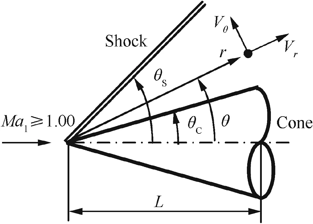
Fig.1 Diagram of a conical shock wave.

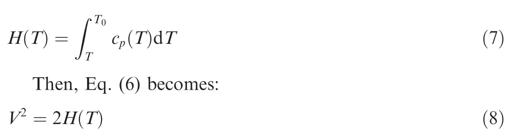
Let us replace Eq.(4)in Eq.(8)and derive the result by the angle θ,replace Eq.(2)and the derivative of Eq.(7)in the result,then replace Eq.(5)in the obtained results,and one obtains:

We assume that the state equation of a perfect gas(p=ρRT)remains valid1,2,5,11–14,23withR=287.102 J/(kg·K).Expressions ofcpandRfor air are presented in Refs.11,12For the PG model,γ=1.402 is taken for calculation.1,11,12

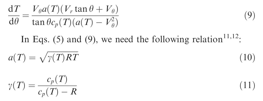
Eqs(2),(5),and(9)constitute a system of three differential equations with three coupled unknowns(Vr,Vθ,andT).Given the complexity of the obtained equations,an analytical solution does not exist.Hence,our interest is directed towards the search for a numerical solution.

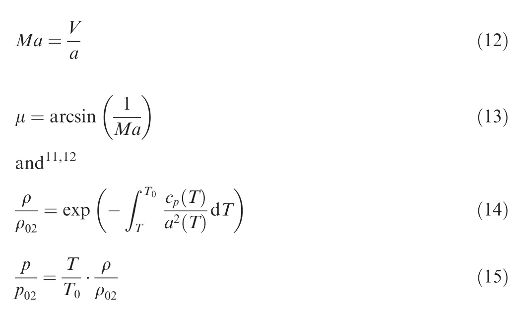
The other parametersV,a,Ma,μ,ρ/ρ02,andp/p02can be determined respectively by Eqs.(4),(10),and the following:

The ratiop02/p01is determined by the calculation of the flow through the conical shock.It is constant between the shock and the surface of the cone as the flow is isentropic in this region.

Eqs(2),(4),(5),(9),(10),(12)–(15)determine the isentropic flow parameters after the shock on the surface of the cone as a function of the angle θ as shown in Fig.1.

3.Numerical procedure

The problem solving of the flow around a cone uses the inverse method,i.e.,it is considered that the deviation of the shock is given and we determine the corresponding cone deviation that will withstand this shock.This is contrary to a direct approach,where the cone deviation is given and the corresponding shock is determined.Then the data of our problem are θSandMa1forT0given for air.That is to say,in addition,it is necessary to know the variation ofcpwith the temperature and the constantRof the air.

The first step consists of determining all the isentropic parameters(T1/T0,ρ1/ρ01,andp1/p01)corresponding toMa1andT0just before the shock using the relations of an isentropic supersonic flow.3,4,7,11,12The integral Eq.(14)is made using the Simpson quadrature with node condensation.11,12,15,24,25

The second step consists of determining the properties of the flow through the shock,which are summarized byMa2,ψ,T2/T1,ρ2/ρ1,p2/p1,p02/p01,and ΔS21,using the following equations of an HT oblique shock wave19–22after making the modifications cited before:

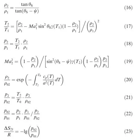
It can be demonstrated that the total temperature through the shock is retained.Then,T0=T01=T02.However,the total pressure and density change values.Hence,p02/p01=ρ02/ρ01≠ 1.0.For the total pressure,p0=p01is set.

Since there is an increase in entropy through the shock,consequently,according to Eq.(23),we will have a decrease in the total pressure across the shock.

Two solutions can be found according to the Mach numberMa2just after the shock,implying that all thermodynamic parameters will admit two solutions.IfMa2≥1.00,a weak shock is obtained.IfMa2＜1.00,a strong shock is obtained.Generally,a weak shock occurs in nature.

Before evaluating the parameters presented in Eqs.(16)–(23),the flow deviation ψ immediately after the shock must be determined.In the Refs.19–22,authors use the relation for a PG model,with constantcp,given the difficulty of finding an analytical form despite nonlinear,which gives results far enough from reality and does not answer the need to an HT model.Then in this work,we will determine the deviation ψ with a high accuracy according to the real HT model.All the parameters after the shock depend directly and explicitly on the value of ψ.Since there is a solution to the problem,the value of ψ ＞ 0.The development of an analytical relation between the parameters θSand ψ is quite complicated;we will use the relations of a normal shock wave at HT26to determine the value ofMa2with other procedures presented in the Ref.21.The relation between the Mach number normal to the shock and the direction ψ is given as follows8,11,20–22:

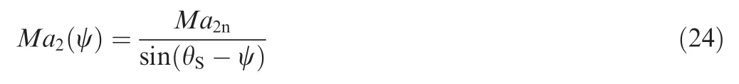
The value ofMa2ncan be found using the procedure presented in the Ref.26It depends onT0andMa1nupstream normal to the shock,equal toMa1sin θS.Therefore,there is no dependence on ψ in the determination ofMa2nby Eq.(24).

The search for the value of ψ is done in such a way that the value ofMa2given by Eq.(24)is equal to the value ofMa2given by Eq.(19).The calculation is done by iteration.For this reason,consider the difference between the value ofMa2given by Eq.(24)and the value ofMa2given by Eq.(19)by the following relation:

Start with ψ = ψG=0.In this case,the value of χG= χ＞ 0.By increasing the value of ψ by a chosen step Δψ,one obtains:

For the value of ψ = ψD,the values ofMa2are calculated respectively by Eqs.(19)and(24),and the difference χDis evaluated by Eq.(25).If the value of χD＞ 0,in this case,the values of ψDand χDare respectively assigned to ψGand χG,and a new value of ψDis calculated by Eq.(26).The calculation will be repeated until we find,for a value of ψD,a value of χD＜ 0.In this case,the physical solution of ψ belongs to the interval[ψG,ψD].We use the bipartition algorithm15,16,24,25to determine the value of ψ,as a solution of Eq.(25),with a given precision χ.For applications,we have taken χ=10-8and Δψ =1.0°.In this case,it is necessary to divide the starting interval[ψG,ψD]to the minimum 21 times.In this step,the value of ψ corresponding to the dataMa1,T0is obtained.By replacing ψ in Eqs.(16)–(23),all the parameters through the shock can be determined.

The third step consists of finding the parameters of the isentropic flow in the region just after the shock and on the cone surface by solving the differential Eqs.(2),(5),and(9)simultaneously by the Runge Kutta method to find at each direction θ,as shown in Fig.1,the parametersVr,Vθ,andT.Then using Eqs.(4),(10),(12),(14)and(15)respectively,V,a,Ma,ρ/ρ02,andp/p02can be calculated.

Among the several orders of the Runge Kutta method that can be found in the Refs.15–18,25,we have used and adapted the fourth Runge Kutta method.In addition to the advantages of this method presented in the introduction,it is very adapted with the presented mathematical model.Order 4 of the method will be sufficient to obtain results with very good accuracy,especially in a reduced execution time in comparison with other orders for the same precision.

The variation domain of the solution is θ ＜ θS.In this case,it is necessary to find θ = θC＜θSto have the solutionVθ=0.In this case,θ= θCcan be replaced by a rigid surface,since the normal velocity is equal to 0.This surface may represent the desired cone surface which supports the given shock.

To allow this method to be used,the initial values ofVr,VθandT2when θ = θSare given by the following equations:

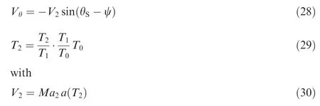
The ratioT2/T1in Eq.(29)is determined during the calculation of the oblique shock in the second step.The ratioT1/T0in Eq.(29)is obtained during the first step when calculating the isentropic parameters corresponding toMa1andT0.The value ofa(T2)in Eq.(30)can be obtained by replacingT=T2in Eq.(10).

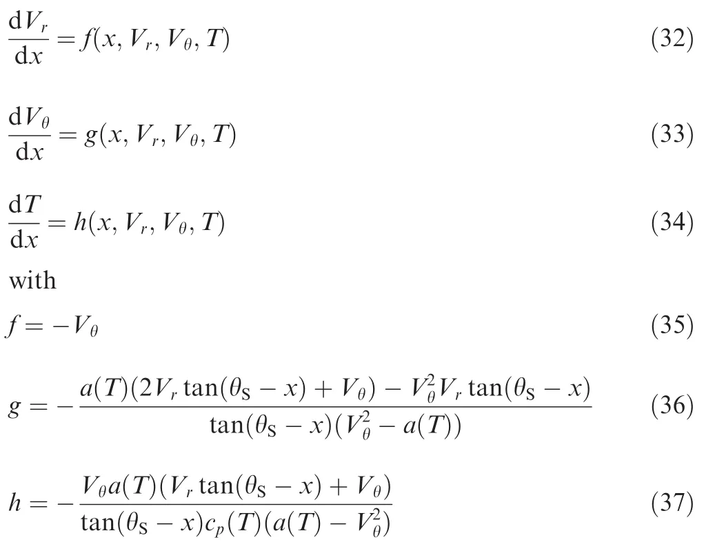
In order to solve the differential Eqs.(2),(5),and(9)in an ascending order,we consider the following change of variable:

The position immediately after the shock θ = θScorresponds tox=0,and the cone position θ = θCtox=xC=θS-θC＞0.Then,the derivative dx=-dθ must be replaced in Eqs.(2),(5)and(9).Then these relations become:

The algorithm of the Runge Kutta method of order 4 to Eqs.(32)–(34)is written as:

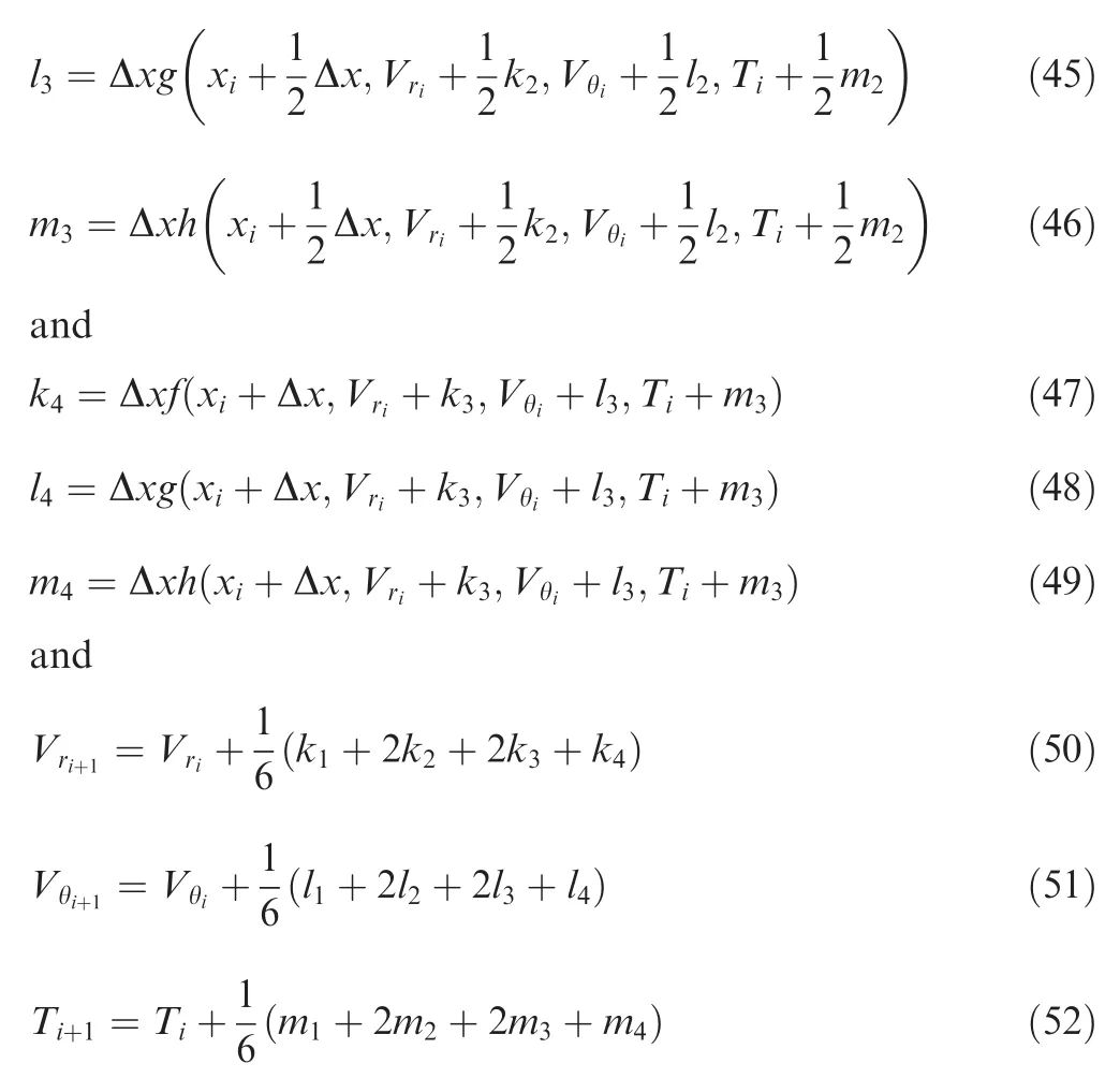
At the initial pointi=0 corresponding to the point just after the shock,Vr,VθandT2take the values given by Eqs.(27)–(29)respectively.At this pointi=0,we haveVθ＜ 0,since it is directed in the opposite direction,as shown in Fig.1.The step Δxmay be constant or variable.In the calculation,a very small constant step has been taken.For each value ofi＞ 0 corresponding to a value ofxi=iΔxand consequently a value of θi= θS-xicalculated by Eq.(31),the parameters can be determined.We need 78 mathematical operations respectively by Eqs.(50)–(52).If other order 4 or even higher-order methods are used,the number of mathematical operations for each step increases,and becomes 283 operations for the method of order 6 while 3314 for the method of order 18.

Then,we can determineVi,ai,Mai, ρi/ρ02,andpi/p02respectively by Eqs.(4),(10),(12),(14),and(15).

It is also possible to determine at each direction θi,the deviation of the velocity vectorViof the flow with respect to the horizon by the following relation:

Wheni=0,the value of α0given by Eq.(53)is equal to ψ.

The results obtained during the calculation can be verified.Since the flow is isentropic after the shock,the parametersMaandTobtained by Eqs.(12)and(52)are related,for our HT model,by the following relation.11,12The same value of the Mach numberMacan be calculated by the following equation and compared with that given by Eq.(12):

The expressions ofH(T)anda(T)in Eq.(54)are given respectively by Eqs.(7)and(10).

The calculation stops if for a value ofi,we findVθ≥ 0.It is rare that we find in the calculation,for a given discretization step Δx,directlyVθ=0.In this case,a refinement of the result or precisely a correction to the value ofxiis made in order to find the solution with a high precision.We therefore use the bipartition algorithm15,16,24,25at the last interval[xi-1,xi].The length of this interval is equal to Δxif the step is constant,or equal to the last step used in the Runge Kutta method.In the calculations,a step Δx=0.001 and an accuracy τ=10-8are used.In this case,the number of subdivisions of the interval[xi-1,xi]is equal to 17.

Once the value ofxwhich cancelsVθis determined,the corresponding cone angle can be determined by Eq.(31),and the values ofV=VrandTcorresponding to the last calculation point represent the values on the cone surface.In this case,the flow parameters such asMa,ρ/ρ02,andp/p02on the cone surface can be found using Eqs.(12),(14)and(15),respectively.

For this last value ofi,the direction of the velocity vector given by Eq.(53)is equal to the corresponding cone deviation.

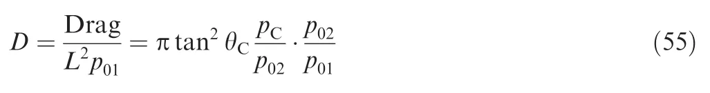
The calculation of the drag force exerted on the surface of the cone is of great interest in aerospace applications.Then,using the Guldin theorem25,it can be demonstrated that the drag developed on the cone surface is given by the following normalized formula:

The physical phenomenon demonstrates that there is a maximum cone deviation θCmaxthat will allow a limit between the attached and detached shock waves.This deviation depends onMa1andT0as well ascpandRof gas.Then if the angle of the cone θC≤ θCmax,there will be an attached shock wave,where the method presented in this study is valid.If θC＞ θCmax,there will be a detached shock wave,and the present study does not give a solution.

The determination of this limit gives us the possibility to avoid the inverse method presented in this study,to consider the solution of the problem by a direct method,where we consider the cone deviation θCamong the data,and to determine the angle of the corresponding shock θS.An additional calculation is made in this case before the corresponding shock determination,since if θC＞ θCmax,the developed program does not give a physical solution to our problem,and a message on the birth of a detached shock wave is presented in this case.Another interesting problem is to determine the minimum Mach number(Ma1min)corresponding to the cone deviation to have an attached shock limit.IfMa1≥Ma1min,we have an attached shock wave;otherwise,a detached shock occurs.This limit depends on θC,T0,cpandRof gas.

It is very convenient for more information and control of the flow to determine the deviation of a cone given a sonic Mach number immediately after the shock(Ma2=1.00)and a sonic Mach number on the surface of the cone(MaC=1.00).The two deviations depend onMa1,T0,cpandR.

By varying the parametersMa1,θSandT0,it is possible to find all the possible parameters,in particular the effect ofT0when it is high.

4.Applications

The phenomenon of conical shock plays a very interesting role in the field of aerospace construction.Several applications can be found.We will brief l y discuss two applications of conical shock.The first application is presented for the adaptation of a supersonic air intake,and the second application is illustrated for the calculation of the wave drag in a wind tunnel test.A third application is presented as a future work.

4.1.Supersonic air intake

An air intake is formed by a nacelle and a central cone that moves between the outside and inside to cause the air intake fitting.This adaptation is necessary,in order not to have degradations of the parameters of the flow,in particular an increase in drag,caused by the reflection of the shock wave in the engine.The adaptation of the air intake is to move the cone axially in a place to have a location of the shock with the hull of the nacelle.The result of displacement depends on the shock deflection and the size of the air intake.Fig.2 shows a schematic diagram of an adapted air intake.The initial position of the cone is given when the cone’s leading edge is placed on the same vertical line as that of the nacelle inlet.

According to Fig.2,for the air intake to be adapted,we can demonstrate that the cone displacement distance must be calculated by the following relation:

The value of θSdepends onMa1,T0and θCfor the air.Then,at high values of theses parameters,the PG model causes the non-adaptation of the air intake.

4.2.Wind tunnel test

The temperatureT0in this case represents the temperature of the combustion chamber formed by the blower.Generally,this temperature is high,which can in most cases exceed 1000 K and reach 3000 K,and influences the parameters found on a prototype(a cone in this case).According to the Ref.14,T0=2100 K for most wind tunnels and aerospace applications.Then,the PG model application gives values that are far from the actual sampling values in tests which are close to those of the HT model,which gives the interest of the present work.

5.Error caused by the PG model

Fig.2 Diagram for an adapted air intake.

The PG model is developed on the basis of considering the specific heatcpconstant,which gives acceptable results for lowT0,Ma1,and θC.According to this study,a difference in the results given between the PG model and our HT model will be presented.The error given by the PG model with respect to our HT model can be calculated for each parameter.Then for each values ofT0,Ma1and θC,the error ε can be evaluated by the following relation:

where ParameterPGand ParameterHTrepresent the values of parameter calculated by PG and HT model,respectively.

6.Results and comments

In this section,the results are divided into 9 parts.All the results obtained are based on three main physical dataMa1,θC,andT0;in particular,one application is made for air.In this case,the functioncpandRfor air are used,although the program can make any gas found in nature.The convergence of the results depends on the discretization which results in the choice of steps used in the Runge Kutta method.In the applications,a step of Δx=0.001 was taken after several convergence tests to obtain an accuracy of χ=10-4.

The results of the conic shock for the PG case(γ=1.402)can be found in the Refs.1–4,8–10

The oblique shock results for the PG model(γ=1.402)can also be found in the Refs.1–4For the HT model,the results presented can be found in the Refs.1,19–22with a moderate difference given the change in the mathematical model in the relationship between the shock deviation and the dihedral deviation and at the level of the interpolation ofcpfor reasons of modeling the HT model with great precision.

6.1.Typical example

Tables 1–9 show all the obtained results by the realized numerical program whenMa1=4.00 and θC=20°by varying the temperatureT0for 1000 K,2000 K,and 3000 K,including the PG case when γ=1.402,to present the effect ofT0respectively on the parameters of weak and strong conical shocks.

Table 1 shows the effect ofT0on the isentropic parameters just before the oblique shock corresponding toMa1=4.00.

Table 2 shows the effect ofT0on the physical parameters through the weak oblique shock whenMa1=4.00 and θC=20°.

Table 3 shows the effect ofT0on the isentropic parameters just after the shock.

Table 4 shows the effect ofT0on the parameters on the cone surface whenMa1=4.00 and θC=20°.It is clear that the isentropic results after the shock(Table 3)as well asMa2(Table 2)are different from those found on the cone surface(Table 4),which shows that the parameters immediately afterthe shock do not remain constant until the cone surface.In Table 4,we added the results for the adapted air intake(value ofC)and those for the wave drag(value ofD)given their importance in practice.

Table 1 Effect of T0on isentropic parameters just before oblique shock when Ma1=4.00 and θC=20°for air.

Table 2 Effect of T0on parameters through weak shock when Ma1=4.00 and θC=20°for air.

Table 3 Effect of T0on isentropic parameters just after weak shock when Ma1=4.00 and θC=20°for air.

Table 4 Effect of T0on parameters on cone surface for weak shock when Ma1=4.00 and θC=20°for air.

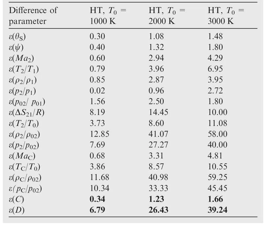
Table 5 Effect of T0on difference between PG and HT models for all conical weak shock parameters when Ma1=4.00 and θC=20°for air.

Table 5 illustrates the error given by the PG model with respect to our HT model on all the parameters calculated in the case of a weak shock whenMa1=4.00 and θC=20°.The influence ofT0on the deviation θSbetween PG and HT is noted.Then the maximum error is noticed for the ratio ρC/ρ02.For the drag,we found an error coming to 39%.In aerodynamics,it is not possible to obtain an error greater than 0.1%between the results given by an observation of nature or an experiment in a wind tunnel and the numerical results presented by the calculation performed.1–5

In Tables 6–9,all the possible results for the case of a strong shock wave for the same example ofMa1=4.00 and θC=20°are shown for information purposes.In fact,there is a great deal of interest in the weak shock,given its appearance in real applications.

6.2.Variations of parameters for remarkable cases

In Tables 10–14,we are interested in the results of very interesting cases in practice for the proposed example ofMa1=4.00 and θC=20°.

It is sometimes very interesting to find the cone deviation givingMa2=1.00 andMaC=1.00 for a givenMa1,and to deduce all the parameters corresponding to these two cases,which demonstrates the interest of the results presented in Tables 11 and 12.The curve corresponding toMa2=1.00 gives the possibility of seeing the disappearance of a strongshock,that is to say,it gives the limit between the strong and weak shocks.The curve corresponding toMaC=1.00 demonstrates the absence of a strong shock on the cone.

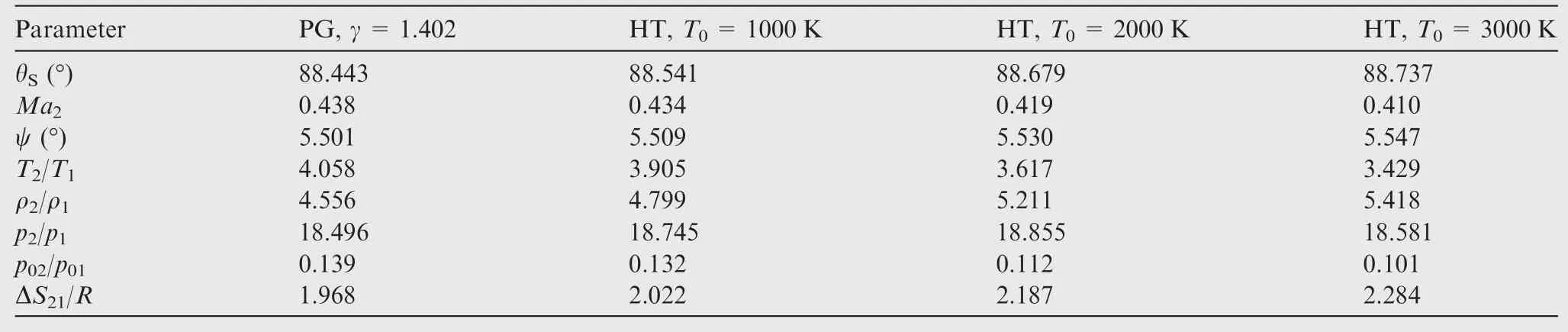
Table 6 Effect of T0on parameters through strong shock when Ma1=4.00 and θC=20°for air.

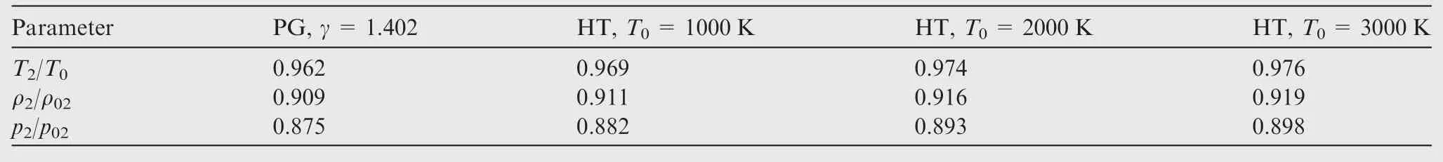
Table 7 Effect of T0on isentropic parameters just after strong shock when Ma1=4.00 and θC=20°for air.

Table 8 Effect of T0on parameters on cone surface for strong shock when Ma1=4.00 and θC=20°for air.

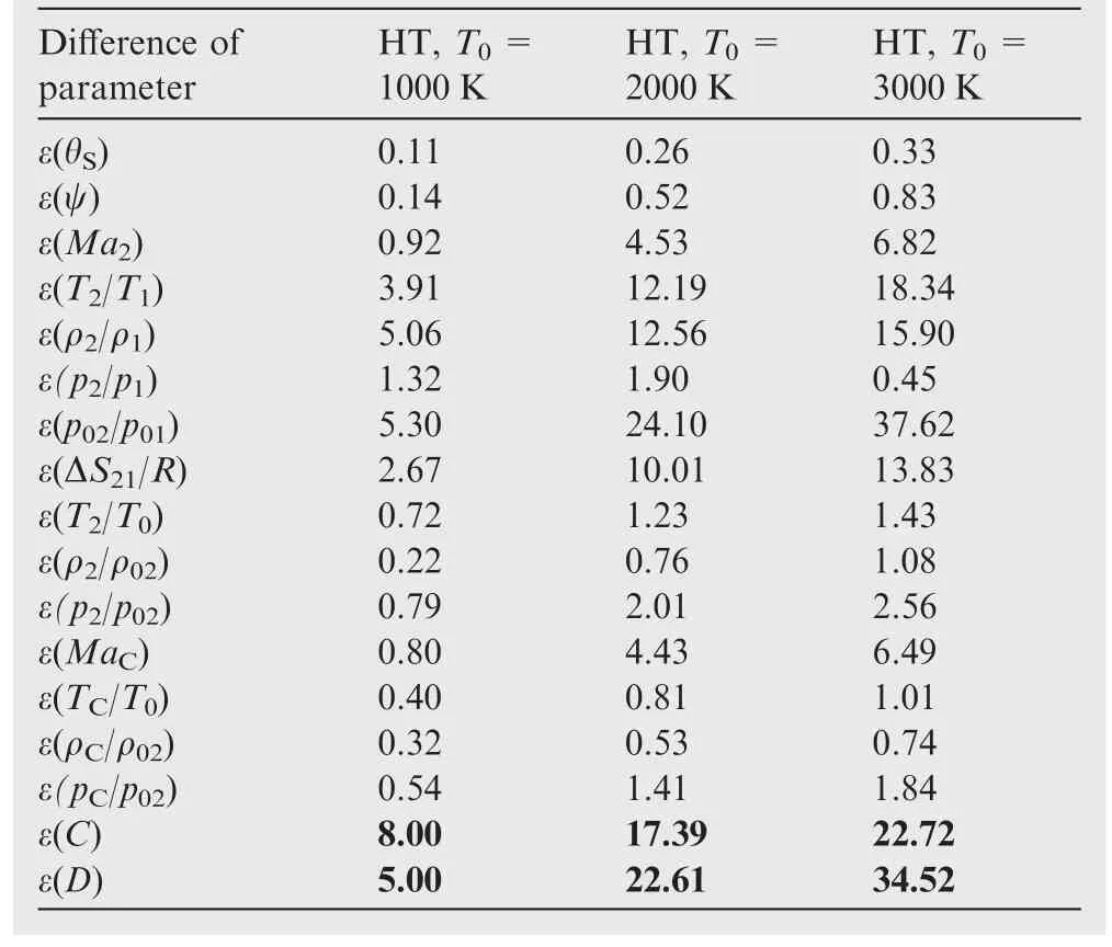
Table 9 Effect of T0on difference between PG and HT models for all conical strong shock parameters when Ma1=4.00 and θC=20°for air.

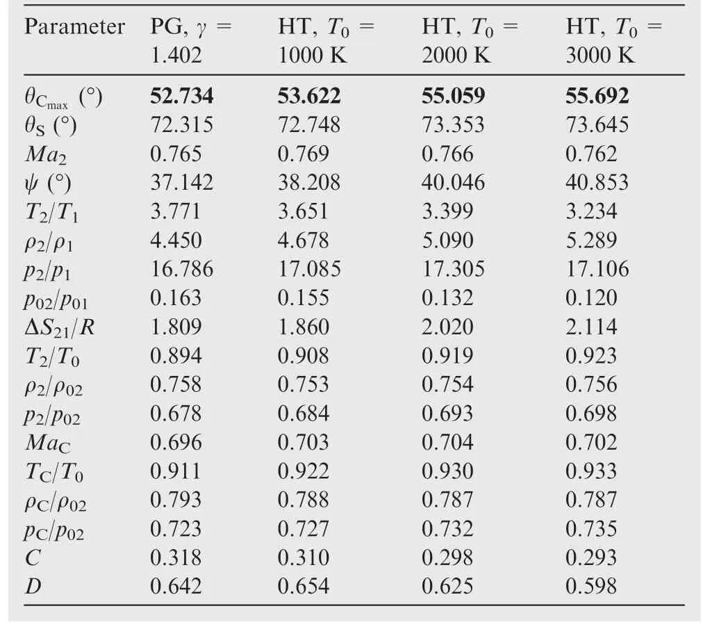
Table 10 Effect of T0on shock parameters corresponding to maximum deviation θCmaxwhen Ma1=4.00 for air.

Table 13 shows the effect ofT0on the minimum valueMa1minof the upstream Mach numberMa1when the cone deviation θCis given to have a boundary between the attached anddetached shocks.In this case,ifMa1≥Ma1min,we will have an attached shock wave.The flow parameters corresponding to θC=20°andMa1=Ma1minare presented for information purposes.

Table 11 Effect of T0on shock parameters corresponding to Ma2=1.00 when Ma1=4.00 for air.

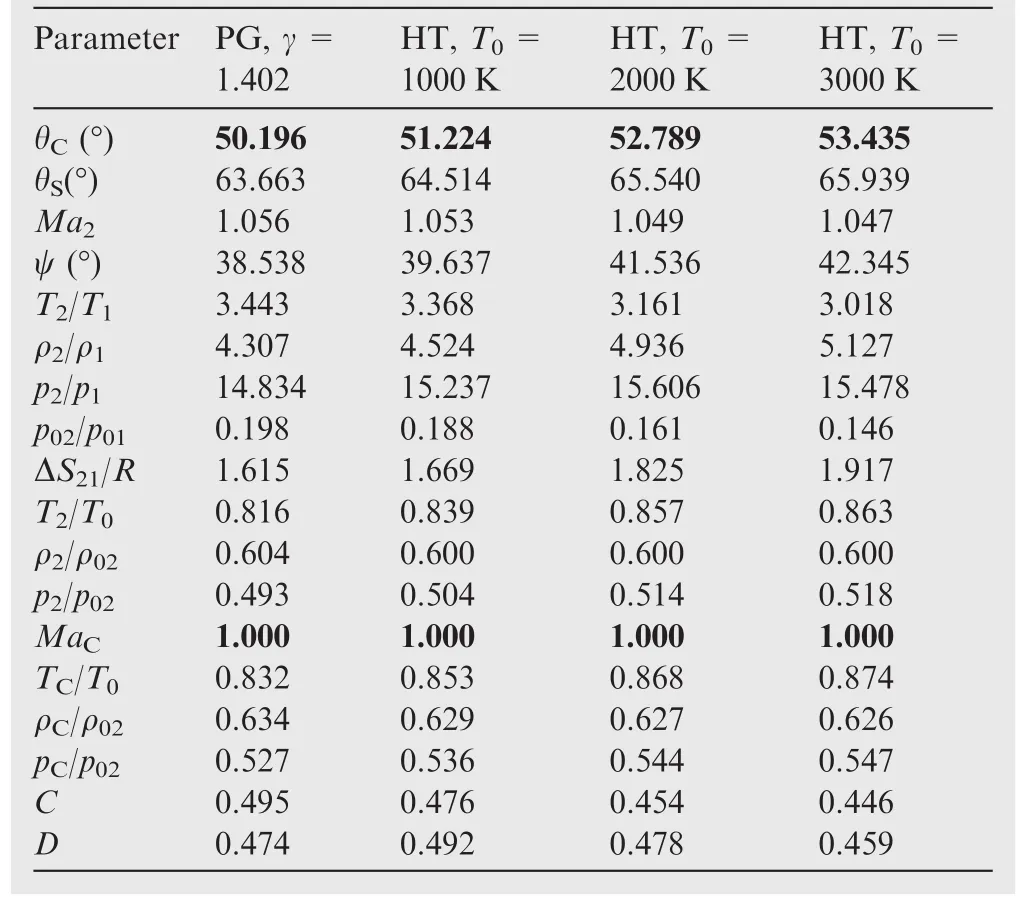
Table 12 Effect of T0on shock parameters corresponding to MaC=1.00 when Ma1=4.00 for air.

In Table 14,the errors between the PG and HT models are presented as a function ofT0respectively for θCmaxandMa1min,and the flow parameters correspond to θC=20° andMa1=Ma1min.

6.3.Variations of parameters as a function of θ

In this third part,Fig.3 show respectively the effects ofT0,including the case of the PG model,on the variations of theisentropic flow parameters(Ma,T/T0, ρ/ρ02,andp/p02)in the region between the shock deviation θSand the cone deviation θCas a function of the angle θ for the weak and strong shocks whenMa1=4.00 and θC=20°.The values of θScan be found from Table 2 for Fig.3(a)–(d)of a weak shock,and in Table 6 for Fig.3(e)–(h)of a strong shock.These figures show that the flow parameters do not remain constant in this region for the cone,unlike for the dihedron19–22,where the parameters after a shock remain constant.The variations of the parameters with θ are valid for someMa1, θC,andT0.The same type of variation of the parameters is noticed between the weak and strong shocks.

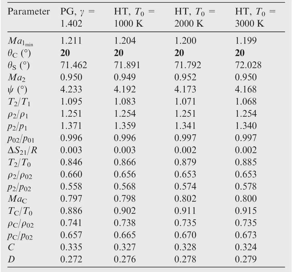
Table 13 Effect of T0on shock parameters corresponding to Ma1minwhen θC=20°for air.

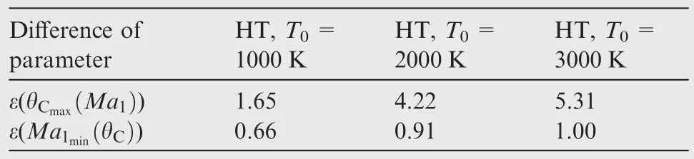
Table 14 Effect of T0on difference between PG and HT models for particular results when Ma1=4.00 and θC=20°for air.

Concerning the developed program,and for plotting Fig.3,the values ofMai,Ti/T0,ρi/ρ02,andpi/p02were not declared in the program for a storage at each flow position θi.Files were used for storing and tracing.

6.4.Variations of parameters as a function of θCfor given values of Ma1when T0is fixed

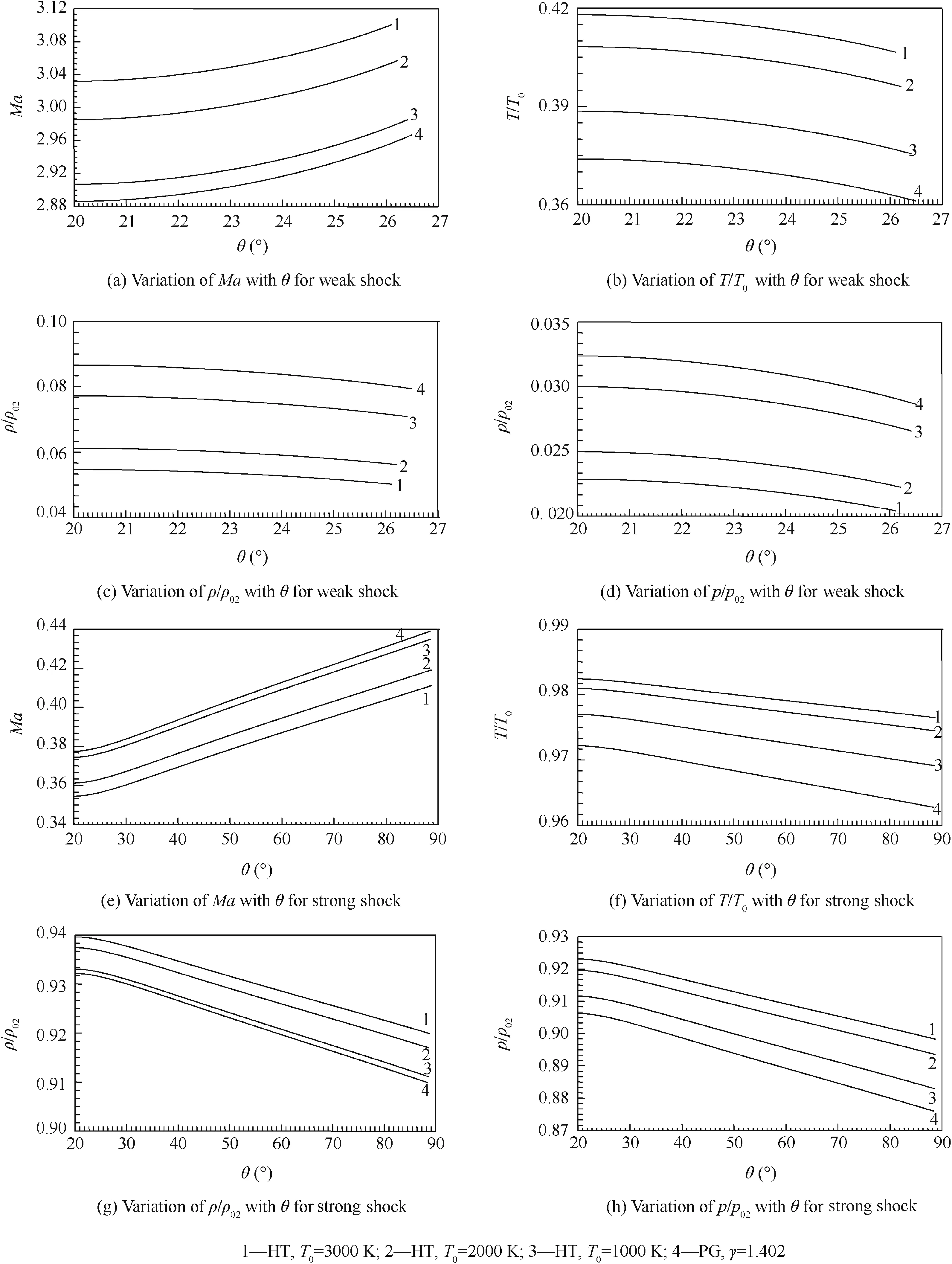
Fig.3 Effects of T0and PG model on variations of isentropic flow parameters for weak and strong shocks when Ma1=4.00 and θC=20°.

Fig.4 show the variations of the physical parameters(θS,Ma2,ψ,T2/T1, ρ2/ρ1,p2/p1,p02/p01, ΔS21/R)through the conical shock.Fig.5 show the varation of the isentropic parameters(T2/T0,ρ2/ρ02,p2/p02)just after the shock.Fig.6 present the variation of the conical surface parameters and Figs.7 and 8 respectively present the variation of the parametersCandD,as a function of the cone deviation θCfor six upstream Mach number values(Ma1=1.30,1.50,2.00,3.00,4.00,5.00)whenT0=2000 K.In each figure,three corresponding curves were added,one for θCmax(to limit the attached and detached shocks),one forMa2=1.00(to limit the weak and strong shocks),and the other forMaC=1.00.For eachMa1,there is one θCmax.

Only in Fig.4(a)which represents the variation of the shock deviation angle with the deviation of the cone,the results for the weak and strong shocks on the same graph have been represented,given the practical interest of this figure.Whereas,for Fig.4(b)–(h)and Figs.5–8,only weak shock results have been shown in the representation,since the addition of the strong shock results renders the presentation bad and condensed.

Fig.4 Variation of physical parameters through conical shock as a function of θCfor some value of Ma1when T0=2000 K.

Between Fig.5 representing the isentropic parameters immediately after the shock and Fig.6 representing the isentropic parameters on the cone surface,it is noted that there is a degradation of the Mach number through the rotation θ,whereMaC≤Ma2,T2/T0≤TC/T0, ρ2/ρ02≤ ρC/ρ02andp2/p02≤pC/p02.It is possible that we findMaC＜1.00 andMa2＞1.00 for the weak shock.

Fig.4(g)shows that the total pressure across the shock decreases with an increase of θC,giving an increase in the entropy according to Fig.4(h),in accordance with the physical shock phenomenon.

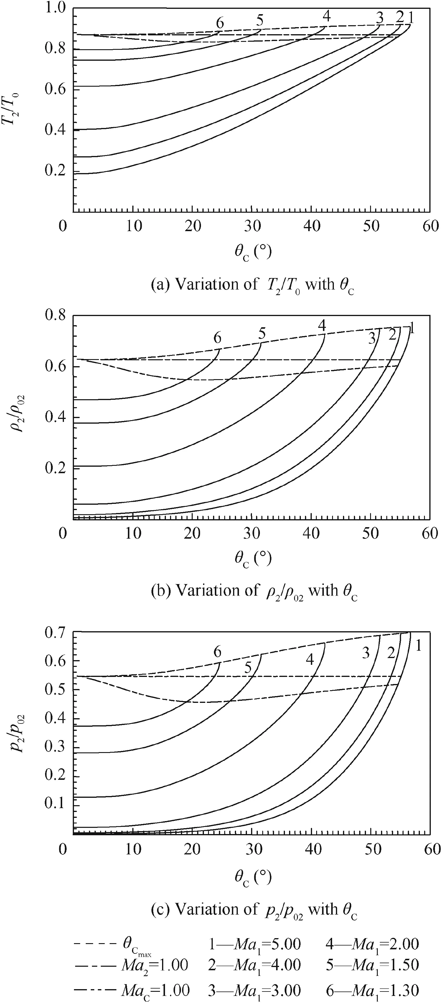
Fig.5 Variation of isentropic parameters after shock as a function of θCfor some value of Ma1when T0=2000 K.

The intersection of each curve ofMa1with the vertical axis,gives two shock possibilities corresponding to θC=0°.In this case,the cone does not exist.The first possibility corresponds to θS=90°which corresponds to a strong normal shock.The results for this HT shock can be found in the Refs.15,17The other lower limit corresponds to the angle of Mach μ given by Eq.(13).The corresponding parameters to the isentropic results before the shock(Ma1,T1,ρ1,p1andp01).In this case,Ma2=Ma1,ψ=0(no dihedron),T2/T1=1.0,p2/p1=1.0,p02/p01=1.0, ΔS21/R=0,T2/T0=T1/T0, ρ2/ρ02= ρ1/ρ01,p2/p02=p1/p01,MaC=Ma1andD=0(no drag).

For the value ofC,according to Eq.(56),it becomes equal for this second limit to the following value:

This last limit does not depend onT0.Comments and variations remain the same for any value ofT0including the PG case.

Table 15 represents the maximum value of the cone deviation angle θCmaxfor the six values ofMa1in Fig.4(a)whenT0=2000 K.These values represent the limit between the attached and detached shocks.

6.5.Variations at HT of parameters as a function of θCfor fixed Ma1

Fig.9 show the effects ofT0including the PG model(γ=1.402)respectively on the variations of all flow parameters(θS,Ma2, ψ,T2/T1, ρ2/ρ1,p2/p1,p02/p01, ΔS21/R,T2/T0, ρ2/ρ02,p2/p02,MaC,TC/T0,ρC/ρ02,pC/p02,C,D)as a function of the cone deviation angle when the Mach numberMa1=1.50,2.00,4.00.Only Fig.9(a)shows the results for the weak and strong shock.While in Fig.9(b)–(q),the presentation was limited only to the weak shock given the poor presentation at the same time of the strong shock.In addition,one is interested practically in the weak shock.

The effects ofT0on all flow parameters are clear,and the difference between the PG and HT models increases further ifMa1and θCincrease gradually.For θC＜ 20°(with an accuracy),we cannot speak about the effect ofMa1orT0.In other words,the PG model can be applied to obtain results with an acceptable precision.However,if θC＞ 20°,the PG model begins to fail by default as corrections to this model are needed which shows the value of the HT model.

Fig.9(g)shows that the total pressure across the shock decreases with increases of θCandMa1giving an increase in the entropy according to Fig.9(h)in accordance with the physical shock phenomenon.

The same remark is now presented between Fig.9(b),(i)–(k)representing the isentropic physical parameters immediately after the shock and Fig.9(l)–(o)representing the isentropic parameters on the cone surface,degradation of Mach number through rotation θ,i.e.,MaC≤Ma2,T2/T0≤TC/T0,ρ2/ρ02≤ ρC/ρ02andp2/p02≤pC/p02.It is possible that we findMaC＜1.00 andMa2＞1.00 for the weak shock.

Table 16 shows the effects ofT0andMa1on the maximum value of the cone deviation angle θCmaxfor the 12 curves in Fig.9.These values represent the boundary between the attached and detached shocks.This precise limit gives the possibility of finding an attached shock solution within the limit given by the PG model,and since this limit gives a detached solution for PG,one will have a possibility of an attached shock solution for HT only ifT0take a rather high value.

The difference between the PG and HT models increases ifMa1also increases with increasingT0and θC.

6.6.Variations at HT of parameters as a function of Ma1for fixed θC

Fig.10 represent the effects ofT0including the case of the PG model(γ=1.402)respectively on the variations of all the flow parameters(θS,Ma2,ψ,T2/T1,ρ2/ρ1,p2/p1,p02/p01,ΔS21/R,T2/T0,ρ2/ρ02,p2/p02,MaC,TC/T0,ρC/ρ02,pC/p02,C,D)as a function of the upstream Mach numberMa1when θC=20°and 40°,respectively.Only in Fig.10(a),the results for the weak and strong shocks are presented,while Fig.10(b)–(q)have limited the presentation for the weak shock given the bad presentation at the same time of the strong shock.In addition,one is practically interested in that weak shock in the reality.

Fig.6 Variation of conical surface parameters as a function of θCfor some value of Ma1when T0=2000 K.

Fig.7 Variation of C of air intake for weak shock as a function of θC.

Fig.8 Variation of drag D of cone for weak shock as a function of θC.

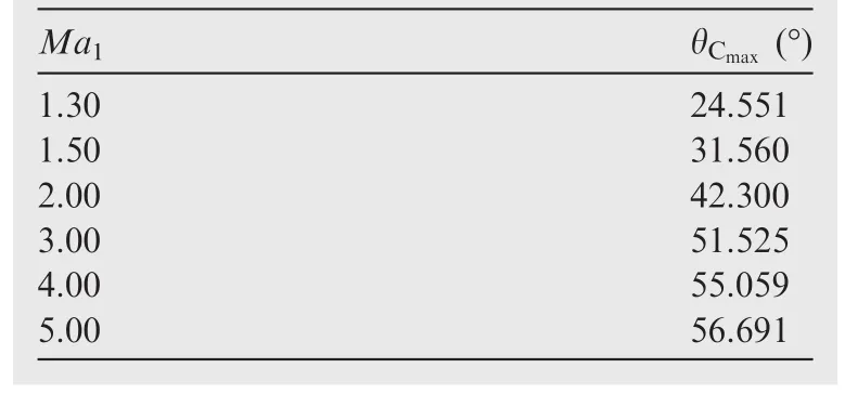
Table 15 Values of θCmaxat HT for some values of Ma1when T0=2000 K.

We clearly notice the effects ofT0on all parameters and the difference between the PG and HT models which increases further ifMa1and θCincrease gradually.For θC＜ 20°approximately,the 4 curves are almost confused(with an accuracy),and one cannot speak about the effects ofT0.In other words,the PG model can be applied to obtain results with acceptable precision.On the contrary,if θC＞ 20°,the PG model begins to fail by default as corrections to this model are needed,which shows the value of the HT model.

It is also noted that ifMa1＜2.00,the 4 curves in Fig.10 are almost confounded independently of the cone angle θC,which demonstrates the possibility of using the PG model for the evaluation of the flow parameters.WhileMa1＞2.00 gradually,the 4 curves begin to separate which shows an increase of the gap between the PG and HT models,which is interpreted by the need to make corrections using the HT model.

Fig.9 Effect of T0and PG model on variations of flow parameters as a function of θC.

Fig.10(g)shows that the total pressure across the shock decreases with increasing θCandMa1,giving an increase in entropy according to Fig.10(h),in accordance with the physical shock phenomenon.

Between Fig.10(b)and(i)–(k)representing the isentropic physical parameters immediately after the shock and Fig.10(l)–(o)representing the isentropic parameters on the cone surface,it is noted that there is a degradation of the Mach number through the rotation θ,i.e.,MaC≤Ma2,T2/T0≤TC/T0,ρ2/ρ02≤ ρC/ρ02andp2/p02≤pC/p02.

Fig.9 (continued)

Table 16 Values of θCmaxfor different Ma1.

Table 17 shows the effects ofT0and θCon the minimum value of the upstream Mach numberMa1minfor the 8 curves in the Fig.10.These values represent the limit between the attached and detached shocks.IfMa1≥Ma1min,there will be an attached shock and a solution of the problem can be found.Then,in Fig.10,the variation ofMa1is betweenMa1min≤Ma1≤5.00.This precise limit still gives a possibility of finding an attached shock solution within the limit given by the PG model,since this limit gives a detached solution for PG,and we will have an attached shock solution for HT ifT0is fairly high.The difference between the PG and HT models increases if θCalso increases with increasingT0andMa1.

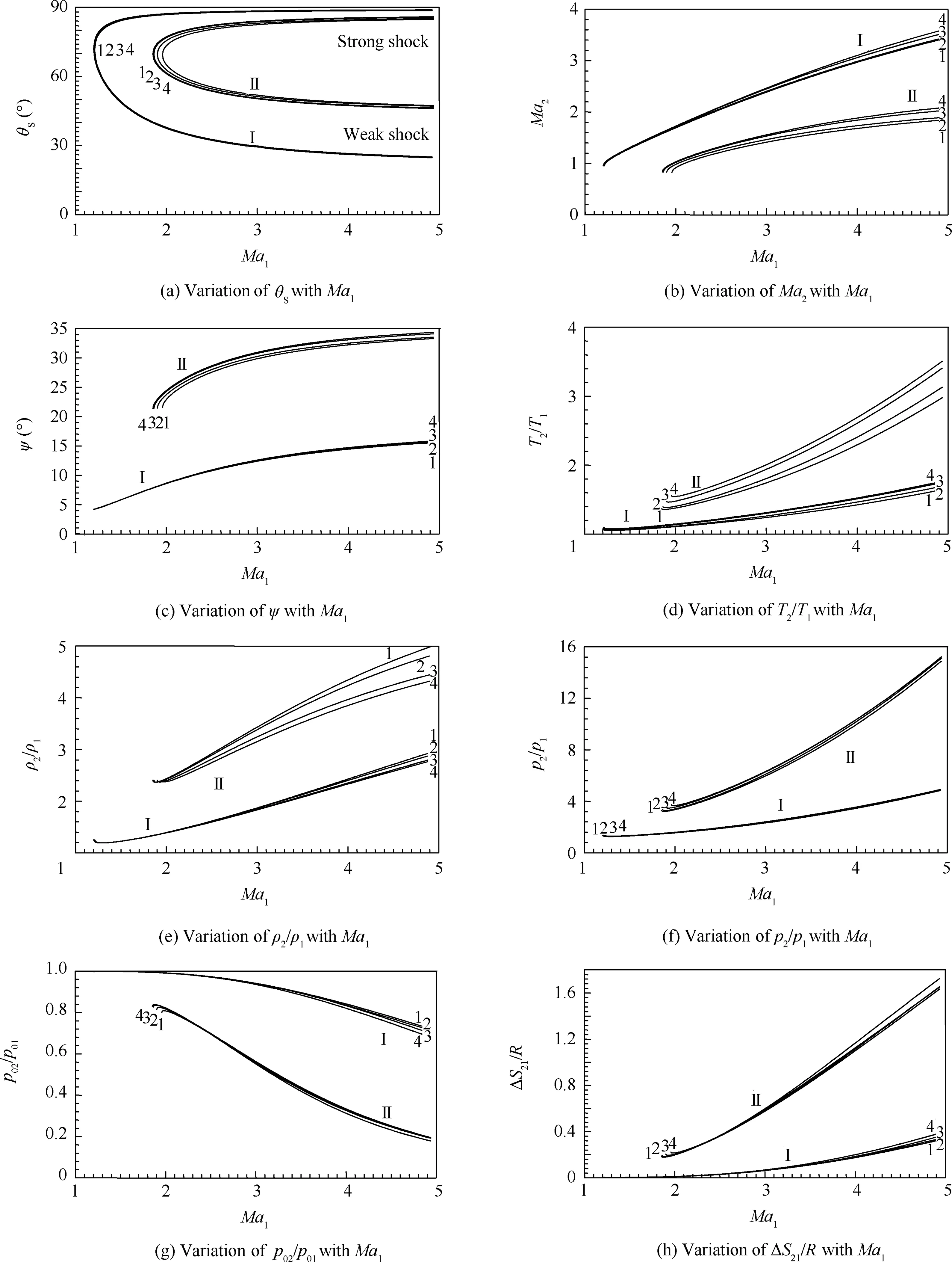
Fig. 10 Effect of T0 and PG model on variations of flow parameters as a function of Ma1.

Fig.10 (continued)

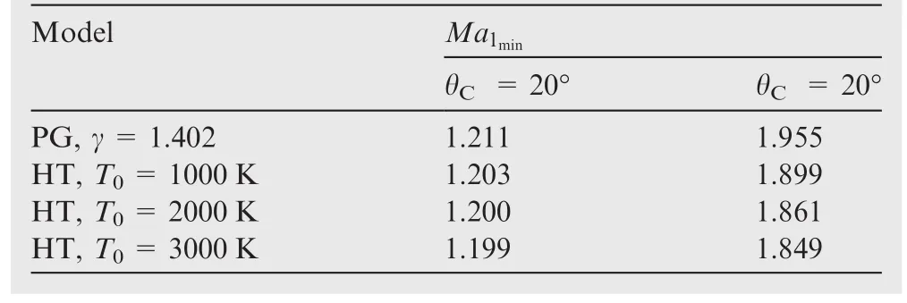
Table 17 Values of Ma1minfor different θC.

6.7.Variations of parameters as a function of T0for fixed θCand Ma1

Fig.11 show the variations of all flow parameters(θS,Ma2,ψ,T2/T1,ρ2/ρ1,p2/p1,p02/p01,ΔS21/R,T2/T0,ρ2/ρ02,p2/p02,MaC,TC/T0,ρC/ρ02,pC/p02,C,D)directly as a function ofT0when θC=20°andMa1=4.00 for the case of the weak shock and a comparison with the PG model(γ=1.402).Note that the PG model does not depend onT0.The flow parameter values for the PG model can be found in Tables 2–4.

Fig. 11 Variation of flow parameters as a function of T0 when θC = 20° and Ma1= 4.00.

Fig. 11 (continued)

The effects ofT0on all the flow parameters are clear,and the difference between the PG and HT models increases asT0increases.ForT0＜240 K approximately,the 2 curves in Fig.11 are almost identical(with an accuracy).In other words,the PG model can be applied to obtain results with acceptable precision.Whereas ifT0＞240 K,the PG model begins to fail by default as corrections to this model are needed,which shows the value of the HT model.

With the same resonance as before,one can make an extension in order to determine a minimum temperature limitT0minwhich will give a limit between the appearances of attached and detached shocks ifMa1and θCare given.

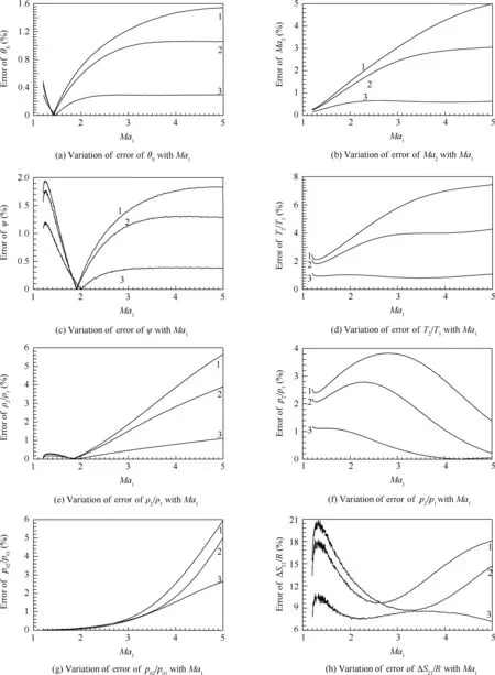
Fig.12 Errors committed by PG model with respect to HT model over all flow parameters as a function ofMa1whenθC=20°forweakshock.

Fig.12 (continued)

6.8.Error of PG model compared to that of HT model as a function of Ma1for θC=20°

Fig.12 represent the errors committed by the PG model with respect to the HT model whenT0=1000,2000,3000 K,respectively,over all the flow parameters as a function ofMa1when θC=20°for the weak shock.We clearly notice the effects ofT0on the relative obtained errors on all the parameters between the PG and HT models.The maximum error of the problem is noted at the ratio ρC/ρ02and is about 90%whenT0=3000 K.For the dragD,it can reach 60%.For the entropy according to Fig.12(h),the error can reach 22%between the two models.For the value ofC,the error can reach 2.0%.In spite of this small error,it can cause a non-adaptation of the air intake since the thickness of the shock wave is very small.

We note that the error increases with increases ofT0and θC,which requires the use of the HT model whenT0is high for possible corrections.For small values ofT0,the PG model gives acceptable results.The PG model usage limit depends on the acceptable accuracy.The errors are presented for θC=20°.Then the calculations made show that the error also increases with an increase of θC.Then for all parameters,the error increases ifT0,Ma1,or θCincreases gradually.The errors found are in agreement with the variations of the results found as a function ofT0,Ma1and θC.

The Mach numberMa1in Fig.12 varies fromMa1=Ma1min(limit between the attached and detached shocks)toMa1=5.00(extreme supersonic).The values ofMa1minfor θC=20°are presented in Table 17.

6.9.Comparison between cone and dihedral

In Fig.13,the angle φ = θCfor the cone equals to φ = ψ for the dihedron.In Fig.13,we have compared all obtained results between the dihedral and the cone whenMa1=4.00 in the case of HT,including the case of the PG model for γ=1.402.Fig.13(a)and(b)shows the results for the weak and strong shocks.However,in Fig.13(c)–(q),the comparison is restricted only to the weak shock.The parameters in the region between the shock and the cone surface depend on the direction θ,and for the dihedral,these parameters are constant and do not depend on θ.Then for the dihedron,we can say thatMa2=p2/p02=pC/p02,while for the cone,these ratios are different.The 4 dotted curves for the dihedron in Fig.13(b)are the same as the 4 curves shown in Fig.13(l);the 4 dotted curves in Fig.13(i)are the same as the 4 dotted curves shown in Fig.13(m);the 4 dashed curves shown in Fig.13(j)are the same as the 4 dashed curves in Fig.13(n);the 4 dihedral curves in Fig.13(k)are the same as those in the dihedron in Fig.13(o).

For φ =0°(isentropic flow)or φ =90°(normal shock wave),the physical parameters for the cone or dihedral are the same.It is noted that the maximum cone deviation corresponding toMa1andT0is greater than the dihedral deviation,which means that there is a bigger attached shock problem solution interval for the cone.

We note again the influences ofT0on all physical parameters also for the dihedral.

The problem of a conical shock is a type of three dimensional problem,while an oblique shock is a type of two-dimensional problem.

In addition,the work is intended for solving conic shock problems with HT,so new results on the HT dihedral are presented as an improvement of the results presented in the Refs.19–22given the modifications made to their mathematical models in this work.

It can be considered that the work carried out can be considered as a numerical wind tunnel.It allows for numerically validating the new HT model with the old existing PG model that is experimentally validated.

As a perspective,this work can be used to study the HT flow around a sharp airfoil obtained by revolution around the longitudinal axis.It is necessary,in this case,to use the Prandtl Meyer relation at HT27,28to evaluate the flow parameters for the case of the expansion.

For a dihedron,Eq.(55)becomes the following form:

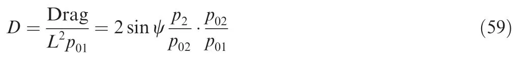
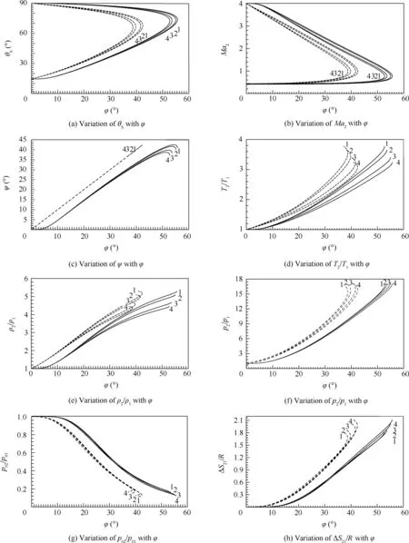
Fig.13 Comparison between dihedral and cone in case of HT and PG model for Ma1=4.00.

Fig.13 (continued)

7.Conclusions

The following conclusions can be drawn from this study:

(1)The PG model gives good results whenMa1＜2.00,T0＜ 240 K,and θC＜ 20°.It disrupts the conical shock performance whenMa1,T0and θCincrease,where the calculation requires the use of our HT model for correction.

(2)The developed numerical program can give results for any gas found in nature.It is necessary to addcpandRof the gas and calculateH(T).The application is made only for air.

(3)The functioncp,Rand γ(T)influence mainly on all the conical shock parameters.

(4)The convergence of the results requires an additional calculation time for our HT model compared to that of the PG model for the same accuracy.

(5)The HT model depends on 4 parameters(Ma1,cp,θC,T0)which gives a generalization of the PG model,and it is represented by 3 nonlinear differential coupled equations with 3 unknowns(Vr,Vθ,T).

(6)WhenMa1,T0or θCis high,the PG model gives a nonadaptation of the air intake and consequently a degradation of its performance.

(7)The flow parameters between the shock and the cone surface depend on the angle θ.

(8)In another external or internal aerodynamics application,the results presented in this study are used in part or in full for the evaluation of this application.

(9)Between all the flow parameters,the maximum error is noticed for ρC/ρ02and can reach 105%whenT0=3500 K for θC=40°andMa1=5.00.

(10)For a givenMa1,if θC≤ θCmax,we have an attached shock wave.Otherwise,a detached shock is observed.θCmaxdepends onT0and the used gas.

(11)For a given θC,if Ma1≥ Ma1min,we have an attached shock.Otherwise,a detached shock is observed.Ma1mindepends onT0and the used gas.

(12)T0is an essential parameter of our HT model.The PG model results do not depend onT0.

(13)T0reduces θS,T2/T1,p2/p1,ΔS21/R,ρ2/ρ02,p2/p02,ρC/ρ02,pC/p02,Dand increaseMa2,ψ,ρ2/ρ1,p02/p01,T2/T0,MaC,TC/T0,Cwith respect to the PG model.This difference increases with an increase ofT0.

(14)The Runge Kutta method of order 4 is used and adapted for solving the system of differential equations.

One can make an extension in order to determine the physical parameters of a shock at high temperature around a pointed cone of an arbitrary 3D section,with zero incidence,at HT,and to make applications for elliptic and polygonal shapes.

Acknowledgements

The authors acknowledges Khaoula Yahiaoui,AbdelGhaniAmine Yahiaoui,RitadjYahiaoui,Assil Yahiaoui,and Mouza Ouahiba for granting time to prepare this manuscript.

1.Hill PG,Peterson CR.Mechanics and thermodynamics of propulsion.Boston:Addition-Wesley;1965.p.250–5.

2.Emanuel G.Gasdynamic:Theory and application.Reston:AIAA;1986.p.155–61.

3.Anderson JD.Fundamentals of aerodynamics.2nd ed.New York:McGraw-Hill;1988.p.137–42.

4.Anderson JD.Modern compressible flow with historical perspective.2nd ed.New York:McGraw-Hill;1982.p.172–9.

5.Sutton GP,Biblarz O.Rocket propulsion elements.8th ed.Hoboken:John Wiley&Sons;2010.p.351–8.

6.Zucro MJ,Hoffman JD.Gas dynamics.Hoboken:John Wiley&Sons;1976.p.226–32.

7.Anderson JD.Hypersonic and high temperature gas dynamics.New York:McGraw-Hill;1989.p.315–21.

8.Maslen SH.Supersonic conical flow.Washington,D.C.:NACA;2002.Report No.:NACA TN 2651.

9.Sims JL.Tables for supersonic flow around right circular cones at zero angle of attack.Washington,D.C.:NACA;1964.Report No.:NASA SP-3004.

10.Chen SX,Li DN.Supersonic flow past a symmetrical curved cone.Indiana Univ Math J2000;49(2):23–31.

11.Zebbiche T,Youbi Z.Effect of stagnation temperature on supersonic flow parameters application for air in nozzles.Aeronaut J2007;16(2):53–62.

12.Zebbiche T,Youbi Z.Supersonic flow parameters at high temperature:Application for air in nozzles.German aerospace congress;2005 Sep 26–29;Friendrichshafen,Germany.2005.p.253–65.

13.Van Wylen GJ.Fundamentals of classical thermodynamics.Hoboken:John Wiley&Sons;1973.p.266–71.

14.McBride BJ,Gordon S,Reno MA.Thermodynamic data for f i fty reference elements.Washington,D.C.:NASA;1993.Report No.:NASA TP-3287.

15.Raltson A,Rabinowitz A.A first course in numerical analysis.New York:McGraw-Hill;1985.p.156–64.

16.Iserles A.A first course in the numerical analysis of differential equations.Cambridge:Cambridge University Press;1996.p.215–29.

17.Butcher JC.On Runge-Kutta processes of high order.J Aust Math Soc1964;4(1):179–94.

18.Luther HA.Further explicit fifth-order Runge-Kutta formulas.SIAM Rev1966;8(4):374–80.

19.Tatum KE.Computation of thermally perfect properties of oblique shcok waves.Washington,D.C.:NASA;1996.Report No.:NASA CR-4749.

20.Neice MM.Table and charts of flow parameters across oblique shocks.Washington,D.C.:NACA;1984.Report No.:TN-1673,1984.

21.Taibi H.Supersonic flow at high temperature on the dihedron[dissertation].Blida:University SAAD Dahlab of Blida 1;2011.p.1–153.

22.Tatum KE.Computation of thermally perfect oblique shock wave properties.Reston:AIAA;1997.Report No.:AIAA-1997-0868.

23.Yahya SM.Gas tables for compressible flow calculation.5th ed.New Delhi:New Age International;2006.p.85–102.

24.De´midovitch B,Maron I.Elements of numerical calculation.Hoboken:John Wiley&Sons;1987.p.121–6.

25.Merzbach UC,Boyer CB.A history of mathematics.3rd ed.Hoboken:John Wiley&Sons;2011.p.184–91.

26.Zebbiche T.Effect of stagnation temperature on the normal shock wave.Int J Aeronaut Space Sci2009;10(1):1–14.

27.Zebbiche T.Stagnation temperature effect on the Prandtl Meyer function.AIAA J2007;45(4):952–4.

28.Zebbiche T.Numerical quadrature for the Prandtl Meyer function athigh temperature with application forair.Thermophys Aeromech2012;19(3):381–4.