Global aerodynamic design optimization based on data dimensionality reduction

Ysong QIU,Junqing BAI,*,Nn LIU,Chen WANG

aSchool of Aeronautics,Northwestern Polytechnical University,Xi’an 710072,China

bAVIC Aerodynamics Research Institute,Shenyang 110034,China

1.Introduction

With the development of high performance computing,aerodynamic shape optimization has been widely used in the process of aircraft shape design. Aerodynamic shape optimization based on Genetic Algorithm(GA)is distinguished from regular optimization by its focus on finding the maximum or minimum over all input values,as opposed to finding local minima or maxima.However,it still faces many challenging problems and issues.One of them is the large num-ber of shape Design Variables(DV)which lead to prohibitive computational cost.Another one is that high-fidelity aerodynamic model based on the Reynolds-Averaged Navier-Stokes(RANS)equations takes up the majority of the overall optimization time.

There are several approaches to deal with large number of design variables.Gradient-based methods with adjoint gradients,1which can efficiently compute gradients without restriction of the number of design variables,have been widely used in aerodynamic shape optimizations.2,3However,gradient based methods are more likely to find local optima especially in multi-modal problems.On the other hand,gradient-free methods are more likely to find the global optimum,but the computational cost is higher when dealing with large numbers of variables.Currently,there are two possible solutions widely used to reduce the number of DVs.One is variable screening4,5which can identify some design variables that contribute to the objective function most and leave out the others to reduce the dimensionality of design space.However,this method will reduce the size of design space and even cannot find the optimal designs that can only be found in original design space.The other is data dimensionality reduction method which can reduce the number of DVs under the precondition of maintaining the generality of original design space.For example,Ghisu et al.6applied Principal Components Analysis(PCA)to reduce the number of DVs in the design of a core compression system for turbofan engine.Similarly,Ghoman et al.7,8studied the application of Proper Orthogonal Decomposition(POD)in multi-disciplinary optimization framework.Toal et al.9,10used POD to filter badly performing geometries and thus reduced the design space.Gao et al.used PCA in many-objective engineering problems.11Besides,some nonlinear data dimensionality reduction methods have been gradually used in aerodynamic shape optimization,such as Generative Topographic Mapping(GTM)studied by Viswanath et al.12,Active Subspace Method(ASM)used by Lukaczyk et al.13and ISOMAP applied by Qiu.14

As for the second problem,namely high computational cost of the CFD solver,there are several methods used in aerodynamic shape optimization.Among all of them,the Surrogate-Based Optimization(SBO)15–17is the most popular since it can build an inexpensive response surface approximation of high-fidelity model.However,when dealing with large number of DVs,the surrogate model approaches become prohibitive since the large number of samples for surrogate model training and tuning processes require huge computational time.Another approach is proposed by LeGresley and Alonso.18–20They applied POD to build Reduced Order Model(ROM)for an inverse design optimization problem.Then Bui-Thanh et al.21,22extended gappy POD to the inverse airfoil design problem which demonstrated a great simplification.Qiu and Bai23proposed POD-surrogate ROM to predict stationary flow fields,which also reduced the computational time in optimization.

The focus of this paper is to reduce the overall computational cost and improve the efficiency of global optimization by data dimensionality reduction method—POD.For this purpose,typical surrogate-based optimization system is introduced in Section 2.In Section 3,POD is applied in dimensionality reduction of design space and acceleration approach for samples calculation in surrogate modeling.The new optimization system is proposed in Section 4 based on the work mentioned above.Following that,the optimizations of a RAE2822 airfoil and ONERA M6 wing are used as test cases to demonstrate the effectiveness of the proposed strategy.Finally,conclusions are drawn in Section 5.

2.Typical aerodynamic shape optimization based on surrogate model

Surrogate-based optimization is the base of our research.This section describes the components of a typical SBO system:aerodynamic shape parameterization method—Free Form Deformation (FFD),high-fidelity aerodynamic analytical method based on solving RANS,kriging surrogate model and genetic algorithm.

2.1.Aerodynamic shape parameterization method

In this paper,we choose to use FFD to parameterize the aerodynamic shape.It was first proposed by Sederberg and Parry24in 1986 based on the idea that an object is elastic and easy to change shapes under the influence of external forces.If the object is enclosed in a framework and external force is applied to the framework to make it deform,the shape of the object would change as well.Thus,we can control the shape of the object by controlling the shape of FFD framework or the position of FFD control points.A detailed introduction to the method can be found in Ref.25.Fig.1 shows the FFD control framework and the deformation of airfoil.

2.2.high-fidelity aerodynamic analytical method based on solving RANS

The accuracy of CFD method is the guarantee of the quality of aerodynamic shape optimization.In this paper,the aerodynamic performance of different aerodynamic configurations is obtained by solving the RANS equation.

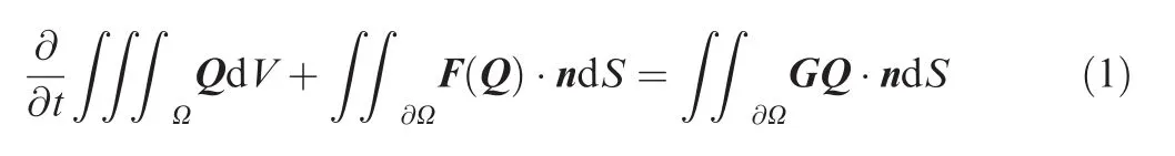
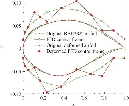
Fig.1 FFD control framework and deformation of RAE2822 airfoil.

where Q is conserved variable,F（Q）is inviscid flux vector,and G（Q）is viscous flux vector;∂Ω is the boundary of control body.Turbulence is modeled using thek-ω Shear Stress Transport(SST)turbulence model.Convergence acceleration is achieved through multigrid.To test the credibility of CFD method,one test case of RAE2822 known as the AGARD test Case 10 is selected.26The external flow condition is Mach numberMa=0.75,Reynolds numberRe=6.2×106,angle of attack α =2.72°.The mesh for the test case and subsequent optimization is shown in Fig.2 and the mesh contains 83000 cells.As seen in Fig.3,the computation predicts the shock wave precisely and agrees well with the experiment data,Cpis pressure coefficient.

2.3.Kriging surrogate model

In this paper,we use kriging surrogate model to predict aerodynamic forces.Besides,for a good estimation throughout the experimental domain,we have chosen Latin Hypercube Sampling(LHS).Kriging surrogate model is widely used in global approximation in simulation-based multidisciplinary design optimization.27Its basic principles are as follows:if there areNsample data X= ［x（1），x（2），...，x（N）］Tand its corresponding values of objective function are Y= ［y（1），y（2），...，y（N）］T(x（i）is anmdimensional vector,mis the number of DVs),kriging surrogate model assumes that the true relationship between the design variables and the objective function values is expressed as

wheref（x）is a determined regression model,z（x）is a stochastic process with variance=σ2and mean value=0.The covariance is defined as

whereRis a function that is closely related to the location of two points x（i）and x（j）in space.It can be denoted as

anddis the weighted distance between two points,namely）

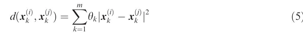
θ can be obtained by maximum likelihood estimation method.

The estimated value^y（x0）of objective functiony（x0）at unknown point x0can be expressed as follows:

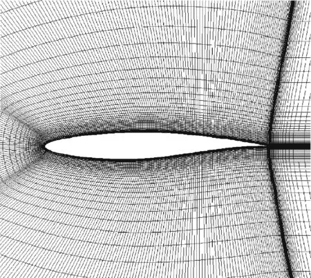
Fig.2 RAE2822 airfoil mesh.

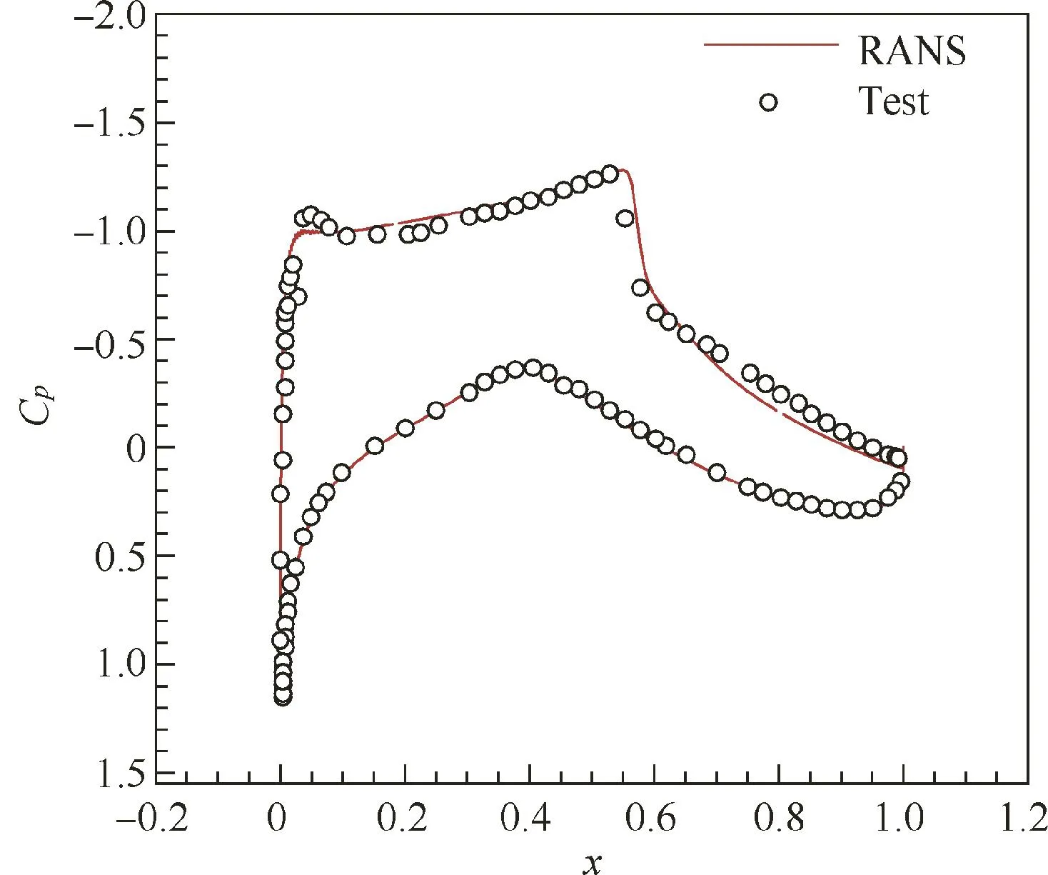
Fig.3 Comparison of pressure coefficients distribution.

where I is unit column vector and rT（x0）is anndimensional vector.is the estimated value of β.and R are as follows:

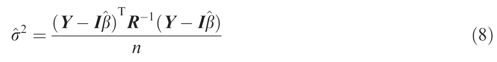
The variance can be written as

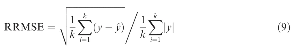
Also,we use the Relative Root Mean Square Error(RRMSE)to evaluate surrogate model accuracy.

2.4.Optimization algorithm

In this work,we use genetic algorithms due to their higher probability of approaching global minimum.Genetic algorithms were first proposed by Holland.28Genetic algorithms are based on natural selection,namely survival of the fittest of Darwinian evolutionary theory.The basic principle is that starting from randomly generated initial population,excellent individuals are selected as the parent based on the survival of the fittest selection strategy.A new generation is generated through selection,mutation and crossover.After many generations of evolution,the fitness of the population will gradually increase.For specific optimization problem,we choose the solution with the highest ranking fitness as the optimum solution.

2.5.Typical surrogate-based optimization system

Based on the components mentioned above,we construct the typical surrogate-based optimization system which is the cornerstone of our research.The flowchart of SBO system is illustrated in Fig.4.

Step 1.Surrogate model training.The initial samples are generated by LHS in the design space.The aerodynamic forces are calculated by high-fidelity CFD solver.Kriging surrogate models are trained based on these training samples.Testing samples are chosen to validate the prediction capability of the model.If it is not precise enough,we need to add more samples to train the surrogate model again.

Step 2.Optimization using GA.We use kriging surrogate model to predict aerodynamic forces instead of high-fidelity CFD solver.Then the current fittest solution of one generation is evaluated by high-fidelity CFD solver and added to the training samples to tune surrogate model until the optimization converges or reaches a plateau without finding a better result.Finally,the optimal solution is output.

2.6.Results and discussion

Before we perform any aerodynamic shape optimization,we first optimize Ackley’s function to explore the impact of dimensionality of design space on the global optimization system.

The Ackley’s function can be expressed as

Fig.4 Flowchart of the basic SBO system.

wherenis the number of input variables andxi∈ ［-10，10］.In its two-dimensional form,as shown in Fig.5,we can see that the design space has multiple local minima although the function is still smooth and the precise global minimumf(x)=0 is found at(0,0).

We use genetic algorithm to minimize Ackley’s function when the number of input variablesn=5,10 and 20.A population of 100 individuals and 100 generations are used while we have considered the following other parameters:probability of crossover=0.9 and probability of mutation=0.1.Surrogate model is not used due to the low computational cost in solving Ackley’s function.The convergence of the optimization algorithm is shown in Fig.6.Asn=5,it needs only about 1000 iterations to find the needle of the global minimum,and asn=10,the iterations come up to 4000.Whenn=20,it is harder for genetic algorithm to converge even after 10000 iterations,which will finally lead to‘the curse of dimensionality’as the number of variables increases.Thus,dimensionality reduction of design space is important to improve the efficiency of global optimization algorithms.

3.Proper orthogonal decomposition

3.1.Principle

In order to reduce the number of DVs while retaining the generality of original design space,we choose data dimensionality reduction method to reduce the dimension of design space.

Proper orthogonal decomposition,29which is also known as kosambi-karhunen-lo’eve decomposition,principal component analysis and singular value decomposition,has been widely used to obtain low-dimensional approximate descriptions of high-dimensional space.

In this work,we apply POD to obtain an optimally orthonormal basis in the least-squares sense for a given set of computational data set used in aerodynamic shape design optimization,like aerodynamic shape parameters,fluid flow variables,etc.The POD method is as follows.30–32

It is assumed that we have a collection of data set as snapshots over a domain Ω,｛Vi（x）:1 ≤i≤N，x ∈ Ω｝,whereNis the number of snapshots.

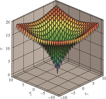
Fig.5 View of two-dimensional Ackley’s function.

Then we decompose the snapshots into a meanV（x）and the fluctuations from this mean

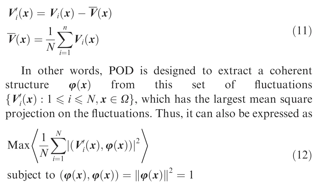
where （·，·）and ‖ ·‖ denote the usual L2inner product and L2-norm over Ω respectively.φ（x）represents the POD basis function and it can be obtained by

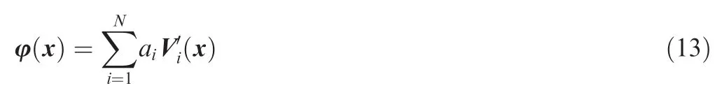
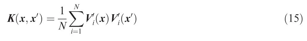
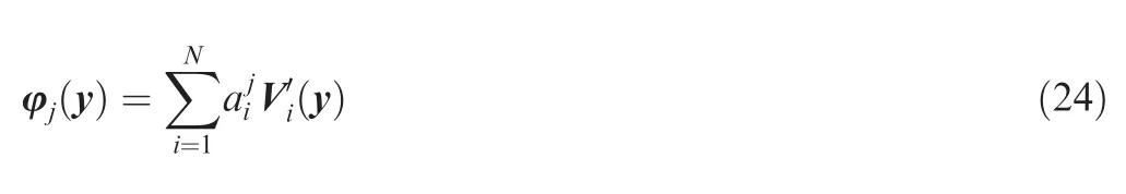
Therefore,the orthogonal basis function φ（x）can be calculated if the coefficientsaiare determined.For this purpose,Ref.29defines

In order to avoid solving a large eigenvalue problem for a full matrix K（x，x′）,Sirovich proposes ‘snapshot’method which overcomes the problem.He defines K（x，x′）as follows:

Thus we just need to solve a matrix K ∈ RN×N.Then,we can obtain the inner product.

As can be seen from the above,the original maximum problem has been transformed into the eigenvalue problem of（Rφ（x），φ（x））.Besides,it has to satisfy the following function in order to maximize （Rφ（x），φ（x））:

Then we can obtain the following equation:

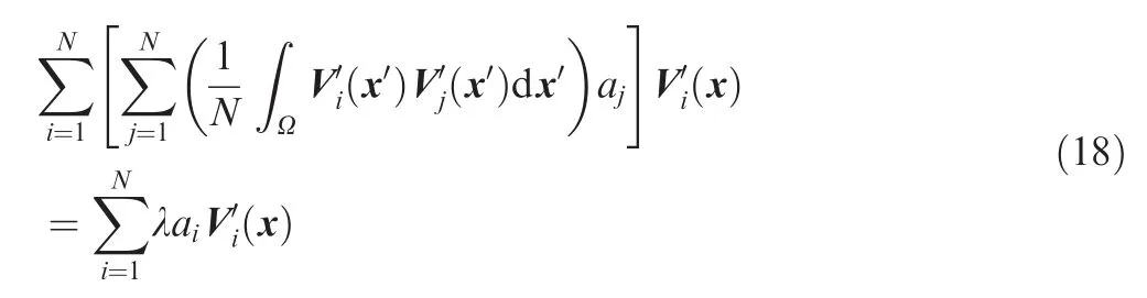
Also,it can be simplified as

Fig.6 Convergence of GA with different Ackley’s function dimensions.

In fact,we do not need all bases to reconstruct the original data set.Since the eigenvalues λ (λ1＞ λ2＞ λ3...＞λN)represent variance,the percent variation explained by the corresponding principal component can be calculated from the respective eigenvalues.Thus,

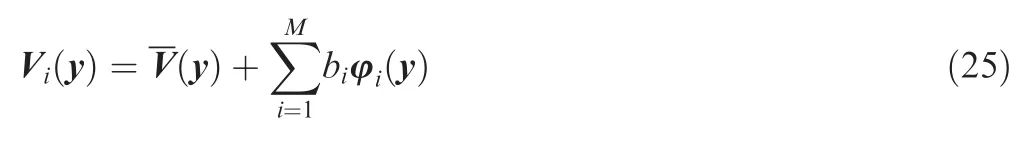
Usually,the first few retain most of the variation or energy present in all of the original variables.The numberMof eigenvalue should be chosen to explain at least about 99%of variation or energy of data set.We can reconstruct the original snapshot vectors as follows:

wherebican be determined through Galerkin projection,30surrogate model23or least square.20

3.2.Dimensionality reduction of design space

Taking airfoil optimization as an example,we apply POD to design space dimensionality reduction which includes the following basic processes:

Step 1.Creating snapshot ensemble.With the help of FFD parameterization,we can obtain a collection of airfoils to construct snapshot ensemble.For airfoil optimization,aerodynamic shape data set of every single airfoil can be expressed as Vi（x，y）.Then we decompose the snapshots into a mean V（x，y）and the fluctuations of each snapshot from this mean.In this work,FFD control points only move in theydirection thus making fluctuations ofxdirection equal to 0.Finally,the POD snapshots can be expressed as（y）.

Step 2.Extracting principal components.We can obtain the nonnegative Hermitian matrix C by

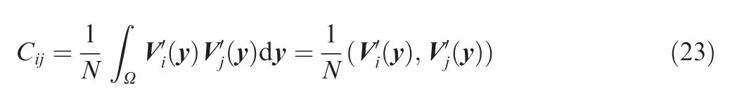
Also,we can get eigenvectors and eigenvalues from matrix C and then choose the firstMeigenvalues which can explain at least about 99%of variation of original data.Thus,we can calculate POD basis by

Step 3.Constructing low-dimensional design space.Take the POD basis coefficientsbias design variables,and the airfoil in the low-dimensional space can be obtained by

3.3.Acceleration approach for samples calculation in surrogate modeling

Another application of POD in this work is to accelerate the solving of steady flow field.In order to reduce the cost of computation in the process of calculation of sampled data used to build surrogate models,especially for optimization with large number of design variables,the acceleration approach for solving a steady flow field through the use of predicted initial flow field has been studied.Based on this approach,the acceleration method has been developed,which divides the process of calculation of sampled data into three stages:in the first stage,a little number is calculated by high-fidelity analysis method;in the second stage,similarity measurement method is used to choose the similar sample as the initial flow field to accelerate the solving of flow field;in the third stage,as the number of samples has been large enough for POD decomposition,POD-surrogate reduced order model is used to predict the initial flow field to accelerate the solving of target flow field.

(1)Similarity measurement method predicting initial flow field

In order to quantify the similarity between two single airfoils,we introduce similarity measurement to describe the affinity–disaffinity relationship between samples.The widely used similarity measurements include Euclidean distance,Manhattan distance,Minkowski distance,Mahalanobis distance,Chebyshev distance,Hamming distance,cosine similarity and so on.

For arbitrary airfoilsa（x1i，y1i）（i=1，2，...，N） andb（x2i，y2i）（i=1，2，...，N）in this work,whereNis the number of airfoil discrete points,thexcoordinates are the same.We can use Euclidean distance to evaluate the similarity of two airfoils:

Through calculation of Euclidean distance between the present airfoil and former samples evaluated with CFD,we can determine the smallest distance and find the most similar airfoil with present airfoil.Therefore,we can take the flow field of the most similar airfoil as the initial flow field for CFD calculation of the target airfoil.23In this way,the computation time can be shortened.However,this method also suffers from some significant problems:only when the initial flow field has been converged,the next CFD calculation which is based on it could converge faster.Also,if there is a great discrepancy between the most ‘similar’airfoil that we find and the present airfoil,the CFD calculation cannot converge or shorten time.

To overcome these problems,we use POD-surrogate reduced order model to predict initial flow field in the third stage once the number of flow field samples has been large enough as snapshot.

(2)POD-surrogate reduced order model predicting initial lf ow field

Taking original variable data set｛ρ，u，v，w，p｝ as the snapshot ensemble（x）,we can obtain principal components:

One thing that we should not overlook is the differences in orders of magnitude among these variables.It is better to extract principal components respectively from every single variable.

Take density field as an example,and the initial density field can be predicted by

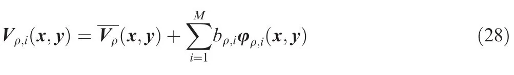
wherebρ，ican be predicted by kriging.

4.New aerodynamic shape design optimization system based on POD

4.1.New optimization system

The effort presented in this work aims to develop a new optimization system based on conventional optimization scheme to improve the overall optimization efficiency,with dimensionality reduction of design space and acceleration approach for solving a steady flow field based on POD.As shown from the flowchart in Fig.7,the new optimization system includes the following basic processes:

Step 1.Dimensionality reduction of design space.A detailed description of this step is presented in Section 3.2.

Step 2.Surrogate model training.We firstly use Latin Hypercube Sampling method to generate sample points in low-dimensional design space for kriging surrogate models.In order to reduce the cost of computation in the process of calculation of sampled data,especially for optimization with large number of design variables,we use the acceleration approach which has also been discussed in Section 3.3.Kriging models are built on these sample points.

Step 3.Optimization using genetic algorithm.

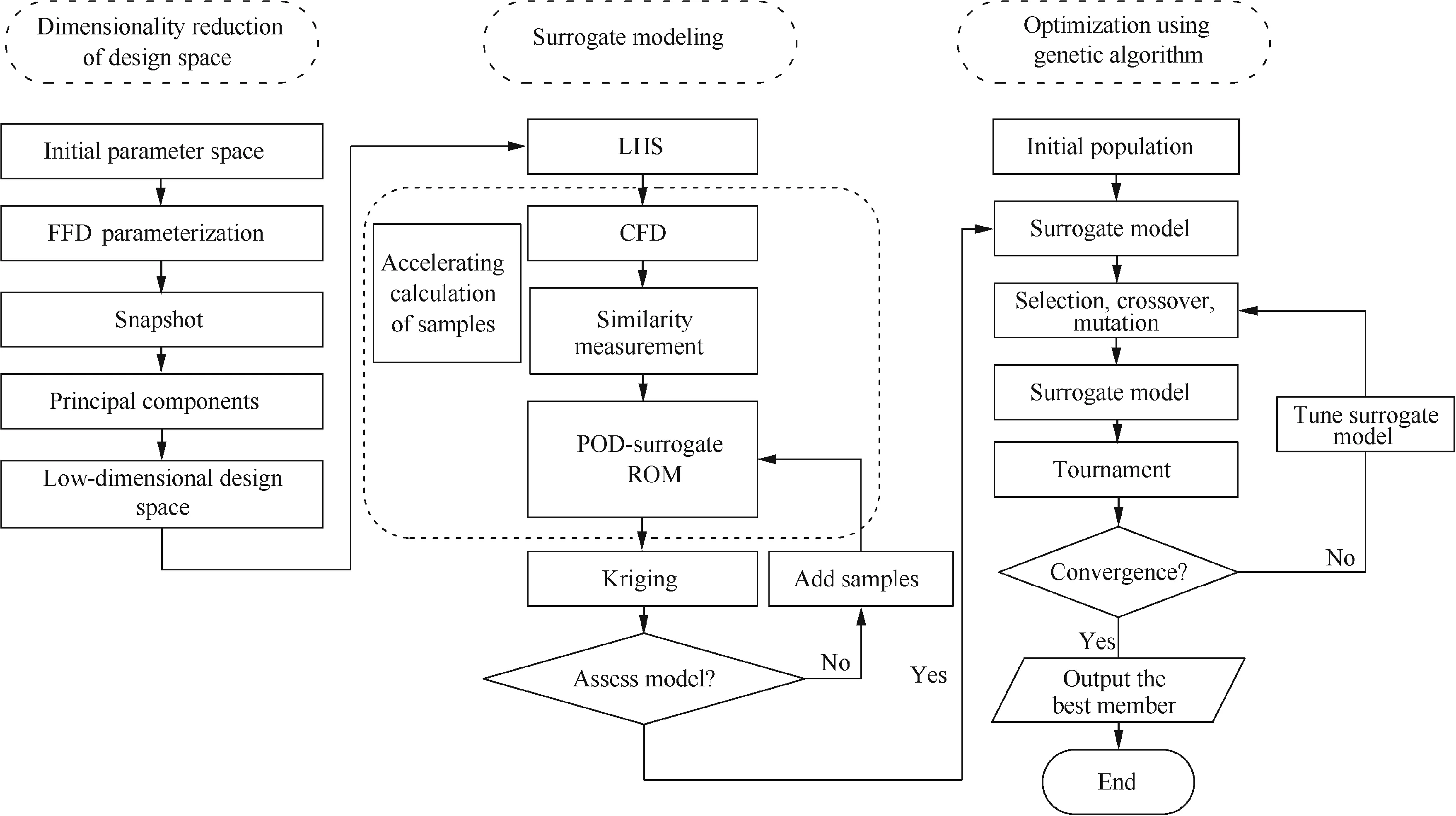
Fig.7 Flowchart of new optimization system.

4.2.Application to transonic airfoil

To demonstrate the effectiveness of the proposed strategy,the optimization of a RAE2822 airfoil is used as a test case.Besides,we also apply the typical surrogate-based optimization strategy for comparison.Both of the optimizations use genetic algorithm.The RANS equations for a compressible viscous flow are solved using the finite-volume CFD code.Turbulence is modeled using thek-ω SST turbulence model.The mesh is the same as that in Section 2.The goal is to minimize dragCDatMa=0.73 andRe=6.5×106subject to a fixed lift coefficient ofCL=0.68.In addition,a relative thicknesst/cconstraint and a pitching moment coefficientCmconstraint are imposed.The optimization problem can be posed as follows:

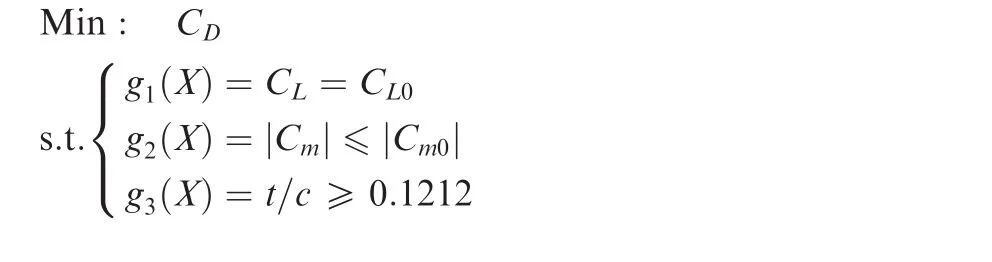
4.2.1.Dimensionality reduction of design space

In the typical surrogate-based optimization strategy,FFD is used to parameterize the airfoil,with 12 FFD control points representing the upper and lower surface respectively,as shown in Fig.8.20 control points are only permitted to vary inydirection while the control points on the leading and trailing edge are fixed resulting in a total of 20 variables.The bound of every design variable is[-0.02,0.02].

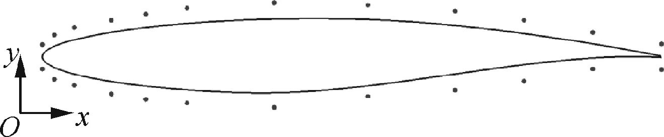
Fig.8 FFD control points of airfoil.

In order to obtain snapshot ensemble for design space dimensionality reduction,a set of 400 airfoils are generated in the original design space by LHS.Every single airfoil includes 280 discrete points,so every airfoil can be denoted as Vi（xj，yj），i=1400，j=1280.As the method mentioned in Section 3.2, we can get the POD snapshotsWe can compute the covariant matrix C according to Eq.(23)and obtain eigenvectors as well as the corresponding eigenvalues arranged in descending order(λ1＞λ2＞λ3＞...＞ λ400).As mentioned earlier,we only need the first few POD basis vectors to construct lower-dimensional design space.In our work,the first 10 POD basis vectors can capture over 99%of the characteristics or energy of the original design space,as shown in Fig.9.

The mean of snapshots and the first 10 extracted mode shapes of the airfoil,which have been added to the mean for visualization purposes,are presented in Fig.10.Through observation of these modes,we can find the following interesting characteristics that are scarcely mentioned in other literature:

(1)The mean of snapshots is similar to original RAE2822 airfoil since all the snapshots are derived from it.Besides,Mode 1 and Mode 2 can be seen as symmetrical about the chord.Mode 3 and Mode 4 can be seen as central symmetric.These laws apply to Mode 5 and Mode 6,Mode 7 and Mode 8,Mode 9 and Mode 10.

(2)As can be seen from the figures,when added up to mean values,the upper surfaces of modes with odd numbers(1,3,5,7,9)change significantly while the lower surfaces nearly do not change.On the contrary,the lower surfaces of modes with even numbers(2,4,6,8,10)change significantly while the upper surfaces nearly do not change.Besides,the eigenvalues of odd number modes are greater than even number modes,so the upper surfaces contribute more to the objective function than the lower surfaces.

Fig.9 Total energy distribution of POD modes extracted from 400 aifoils.

(3)The eigenvalues of Modes 1 and 2 are the greatest among all of the modes.Added up to the mean value,the upper surface thickness of Mode 1 changes significantly while the lower surface nearly doesn’t change,so Mode 1 contributes to the thickness of upper surface most.Similarly,Mode 2 affects the thickness of lower surface most.

(4)In the same way,Modes 3 and 4 and other modes seem to represent other design variables,like leading edge,trailing edge and camber.With the increase of the number of mode,there are more sharply changing zones on the upper surface of airfoil.Also,as the eigenvalues increase,the modes contribute less to the objective function.

Taking the POD basis coefficientsbias design variables,we can obtain airfoil aerodynamic shape in the low-dimensional space according to Eq.(25).Therefore,we manage to move from a surrogate-based optimization based on the original 20 design variables to the one that considers 10 POD basis coefficients.The bounds of the new shape design variables can be determined by the maximum and minimum modal coefficients of the original snapshot ensemble,as showed in Table 1.

4.2.2.Acceleration approach for samples calculation in surrogate modeling

We firstly use Latin Hypercube Sampling(LHS)method to generate 300 samples in new design space.Then we need to run CFD simulation to obtain aerodynamic performance at these sample points.Surrogate models are built on these sample points.The CFD simulation is carried out on a Windows server using Intel(R)Xeon(R)CPU E5-2620 v3@2.40 GHz,with a total of 2 nodes,12 cores per node.In order to reduce the cost of computation in the process of sampled data calculation,we apply the following acceleration approach:

Fig.10 The first 10 POD modes.

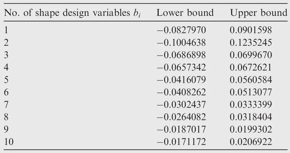
Table 1 New shape design variables for RAE2822 airfoil.

(1)The first 10 samples are calculated by high-fidelity CFD analysis solving RANS equations.

(2)From the 11th to 100th sample,we use similarity measurement method to choose the similar sample as the initial flow field to accelerate the solving of flow field.

(3)From the 101st to 300th sample,we use POD-surrogate reduced order model to predict the initial flow field to accelerate the solving of flow field.

In the second stage,we take the 71st sample as an example.Through calculating the Euclidean distance between the 71st sample and the 70 samples,we find that the 37th sample is the most similar to the target sample.Fig.11 presents the comparison of these two airfoils.The calculation of the 71st sample starts from the 37th sample’s flow field.For comparison of the accuracy and computational cost,we also calculate the 71st sample directly by CFD solver.The results are summarized in Table 2.At the target lift coefficient ofCL=0.68,we can see that the computedCDof two methods are equal to 3 significant digits and 4 significant digits for|Cm|.

In Fig.12,the residual plot shows that the residual(vertical axis)of full order CFD,which uses multigrid method to improve the convergence,reaches a level of 10-9after approximately 67 s and 3000 iterations,while the residuals of similarity measurement method which starts from a previous solution reach the same level after just 400 iterations.The computational time used by similarity measurement method is only 1/4 of the full order of CFD,thus improving the efficiency of CFD computations greatly.

Fig.13(a)and(b)are the convergence history ofCDandCmrespectively.For visualization purposes,the plot only shows the last 1000 iterations of full order CFD calculation results.The comparison of surface pressure distribution and Mach numberMacontour are shown in Fig.13(c)and Fig.14 respectively.The calculatedCpand Mach number of the 71st sample by similarity measurement acceleration method are nearly the same as those by full order CFD.

After the second stage of acceleration,we now have the flow field results of the first 100 samples,which can be used as snapshot ensemble,and then we can construct the POD-surrogate reduced order model to predict the initial flow field of arbitrary airfoil shapes.For the RANS equations,we use original variable data set｛ρ，u，v，p｝ as the snapshot ensemble.Through the method presented in Section 3.3,we can get the POD basis modes respectively from every single variable.As shown in Fig.15,the first 50 POD basis modes can capture over 99%of the total energy of the 100 observations.

Take density field as an example,and the first 6 basis modes can be seen from Fig.16.It is interesting to note that with the number of mode increasing,there are more sharply changing zones on the upper surface of airfoil.The reason is that,due to the presence of shock waves on the upper surface,it is decomposed into every single mode and presented in the density field.

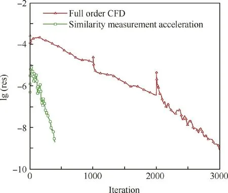
Fig.12 Comparison of residual convergence.

Table 2 Comparison of computational cost and accuracy between full order CFD and similarity measurement acceleration.

Fig.13 Comparison of results of two different simulation methods.

Fig.14 Mach number contour comparison between full order CFD and similarity measurement acceleration.

Fig.15 Total energy distribution of POD modes extracted from 100 sample flow fields.

In the third stage,we take the 193rd sample as an example to accelerate the convergence of its flow field.We predict the mode coefficient by kriging surrogate model and then combine the mode coefficient with POD basis modes as Eq.(28)to predict the initial flow field.It takes only 2.5 s to assemble the basis modes.The calculation of the 193rd sample starts from the approximate initial flow field.Also,for comparison of the accuracy and computational cost,we also calculate the 193rd sample directly by CFD solver.The results are summarized in Table 3.At the target lift coefficient ofCL=0.68,we can see that the computedCDandCmof two methods are equal to 4 significant digits.

With the same convergence tolerances,as shows in Fig.17(a),the full order CFD method takes 3000 iterations and 67 s,while the POD-surrogate ROM only needs 500 iterations and 20 s.

Fig.17(b)and(c)are the convergence history ofCDandCmrespectively.For visualization purposes,the plot only shows the last 1000 iterations of full order CFD calculation results.Due to the predicted initial flow field including less viscous information,the calculation starts from the previous solution with higher numerical oscillations and it still converges faster than full order CFD.

The comparison of pressure contour is shown in Fig.18.The predicted pressure distribution and pressure contour are a little different with full order CFD solutions.By running CFD calculation on the coarse solution,the final calculatedCpby similarity measurement acceleration method is nearly the same as full order CFD.

POD-Surrogate ROM acceleration method can predict the approximate flow field as initial solution thus avoiding choosing inappropriate solution which may lead to slower convergence.With just around 500 iterations,we can obtain the final flow field.With the same convergence tolerances,the computational time used by POD-Surrogate ROM acceleration method is only 1/3 of that used by the full order CFD,thus improving the efficiency of CFD computations greatly.

Fig.16 The first 6 density modes.

Table 3 Comparison of computational cost and accuracy between full order CFD and POD-surrogate ROM method.

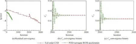
Fig.17 Comparison of results between full order CFD and POD-surrogate ROM acceleration method.

With the acceleration approach mentioned above,we can finish the calculation of all sampled data used to build surrogate models at a much lower computational cost.Besides,the computational time of acceleration approach for solving the flow field of all the 300 samples is only 2 h and 11 min while the full order CFD needs 6 h.

After establishing the surrogate model with the training samples,an effort is made to validate the prediction capability of the model beyond the set of training samples.Another 50 testing samples which serve as a model validation objective are obtained from the low-dimensional design space.The predicted force coefficientsCDandCmagree well with the results calculated by full order CFD,as can be seen in Fig.19.The RRMSEs forCDandCmare 2.31%and 3.16%respectively.

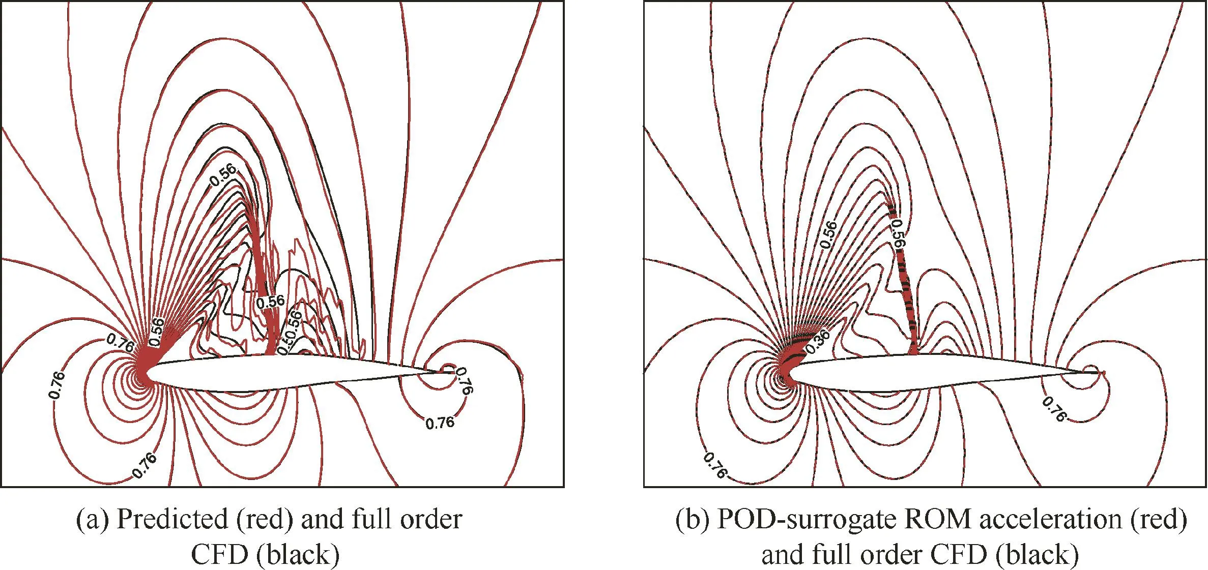
Fig.18 Comparison of pressure field between different methods.

Fig.19 Comparison of surrogate model prediction and calculated results by full order CFD.

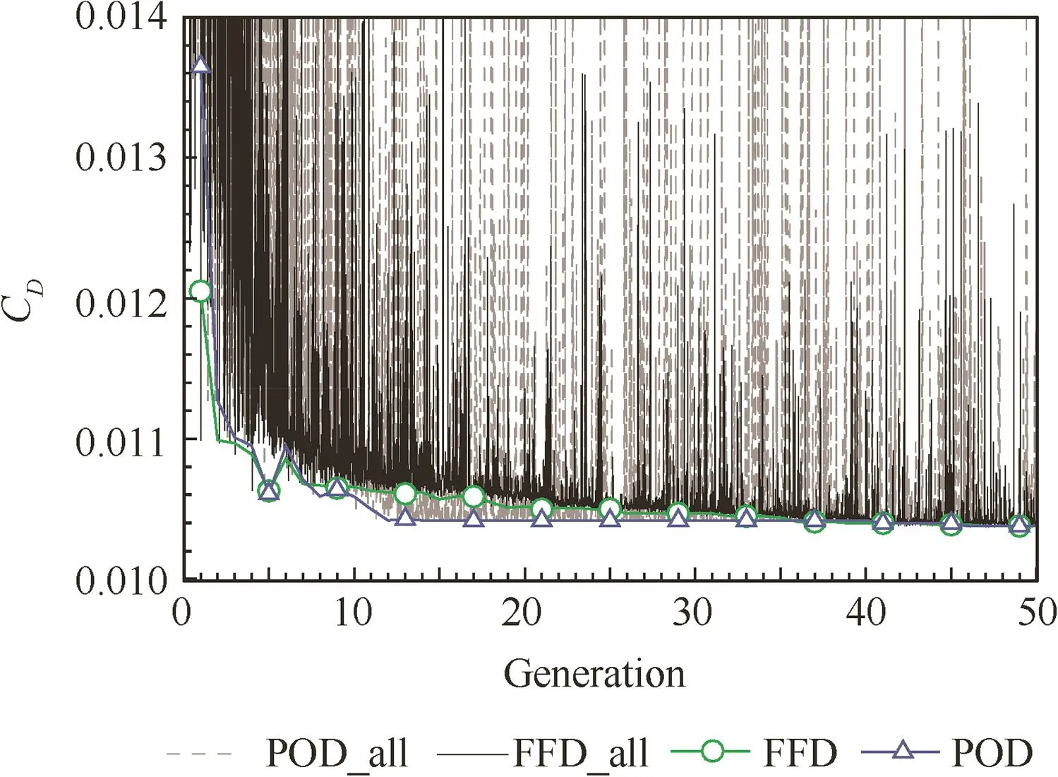
Fig.20 Convergence histories of typical surrogate-based optimization(denoted by FFD in the figure below)and new optimization system(denoted by POD in the figure below).

As mentioned earlier,two optimizations are considered.One is new optimization system constructed in our work and the other is typical surrogate-based optimization.The design variables of typical surrogate-based optimization are 20 FFD control points.With 600 training samples generated by LHS in the design space and full order CFD evaluating at these samples,we construct the surrogate model and then evaluate with another 50 testing samples.The RRMSEs forCDandCmare 2.14%and 2.82%respectively.

4.2.3.Optimization results and discussion

An effort is made to compare the results and computational cost of the two different optimizations.Both optimizations use GA,and a population size of 5 times the number of design variables through 50 generations.Other parameters are used as follows:probability of crossover=0.9 and probability of mutation=0.1. The convergence histories of typical surrogate-based optimization(denoted by FFD in the figure below)and new optimization system(denoted by POD in the figure below)are shown in Fig.20.The figure includes the result of every individual and the best of each generation which shows the new optimization system with fewer design variables converges much faster.

The optimization results are shown in Table 4.At the optimum,the lift coefficient target and the constraint of pitching moment are met.We achieve a drag reduction of 13 counts as compared with the baseline airfoil.The total drag reductionof new optimization system is larger than the reduction of typical surrogate-based optimization.The difference between two optimization results is due to the different size of design variables.This phenomenon can also be found in other cases,like the case of Ackley’s function.In the limited generations and populations,the larger the size of DVs is,the harder it is for GA to converge or find a better solution.

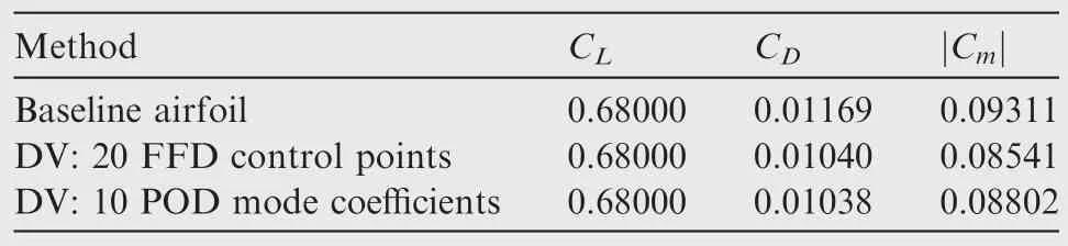
Table 4 Performance comparison.

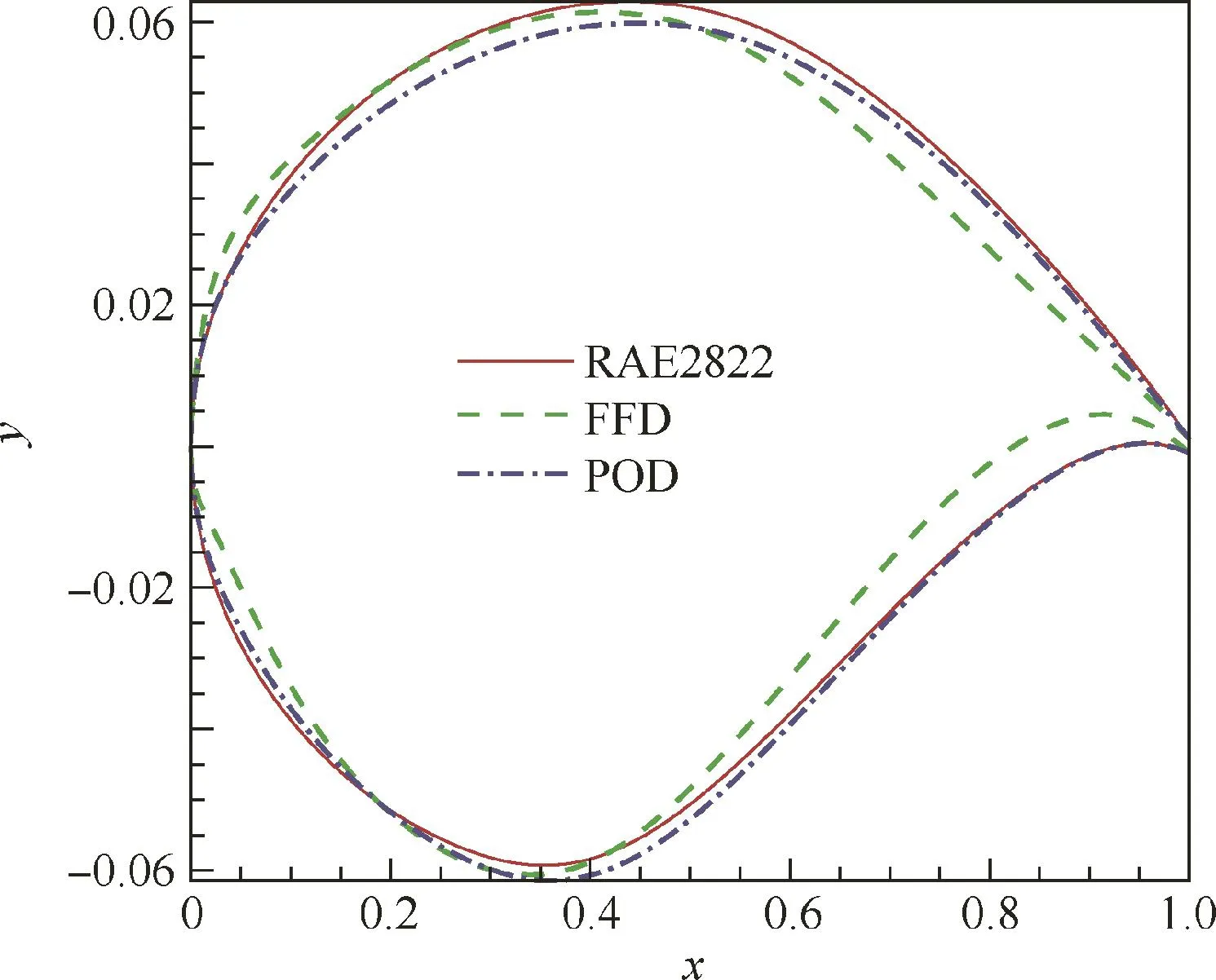
Fig.21 Comparison of both final optimal airfoils and baseline airfoil.

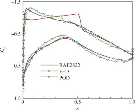
Fig.22 Comparison of pressure coefficients.

Table 5 Computational cost summary.

Fig.21 shows the final optimal airfoils and baseline airfoil.Besides,comparison of surface pressure distribution is shown in Fig.22.Compared with the baseline,the optimized airfoil by typical surrogate model(denoted by FFD in the figure below)has shape changes near leading edge and the aft end,thus making increased loading at both fore and aft lower surface.The optimized airfoil by new optimization system(denoted by POD in the figure below)has a smaller leading edge radius and a flatter upper surface.Besides,as can be seen from Fig.22,both of the optimum airfoils have nearly the same pressure peak near the nose.Fig.23 also shows the comparison of Mach number contour,and the baseline airfoil has a strong shock on the upper surface.It is interesting to note that the optimized airfoil by new optimization system does not show shocks under the design condition while the optimized airfoil by typical surrogate-based optimization has a weak shock on the upper surface.Due to the clustering of shape design variables(20 FFD control points),the genetic algorithm finds it harder to eliminate the shock wave within 50 generations.On the contrary,the dimensionality reduction of design space improves the efficiency of genetic algorithm.

Fig.23 Comparison of Mach contour between original airfoil and two optimized airfoils.

Fig.24 ONERA M6 wing mesh.

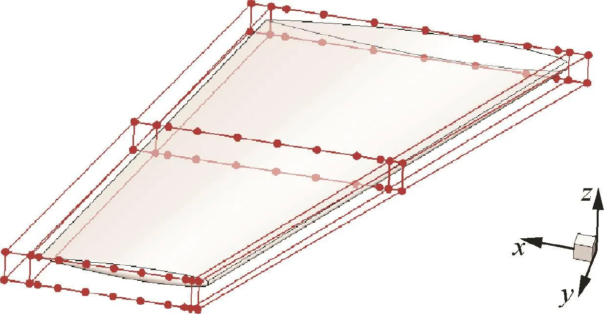
Fig.25 FFD control volume of ONERA M6 wing.

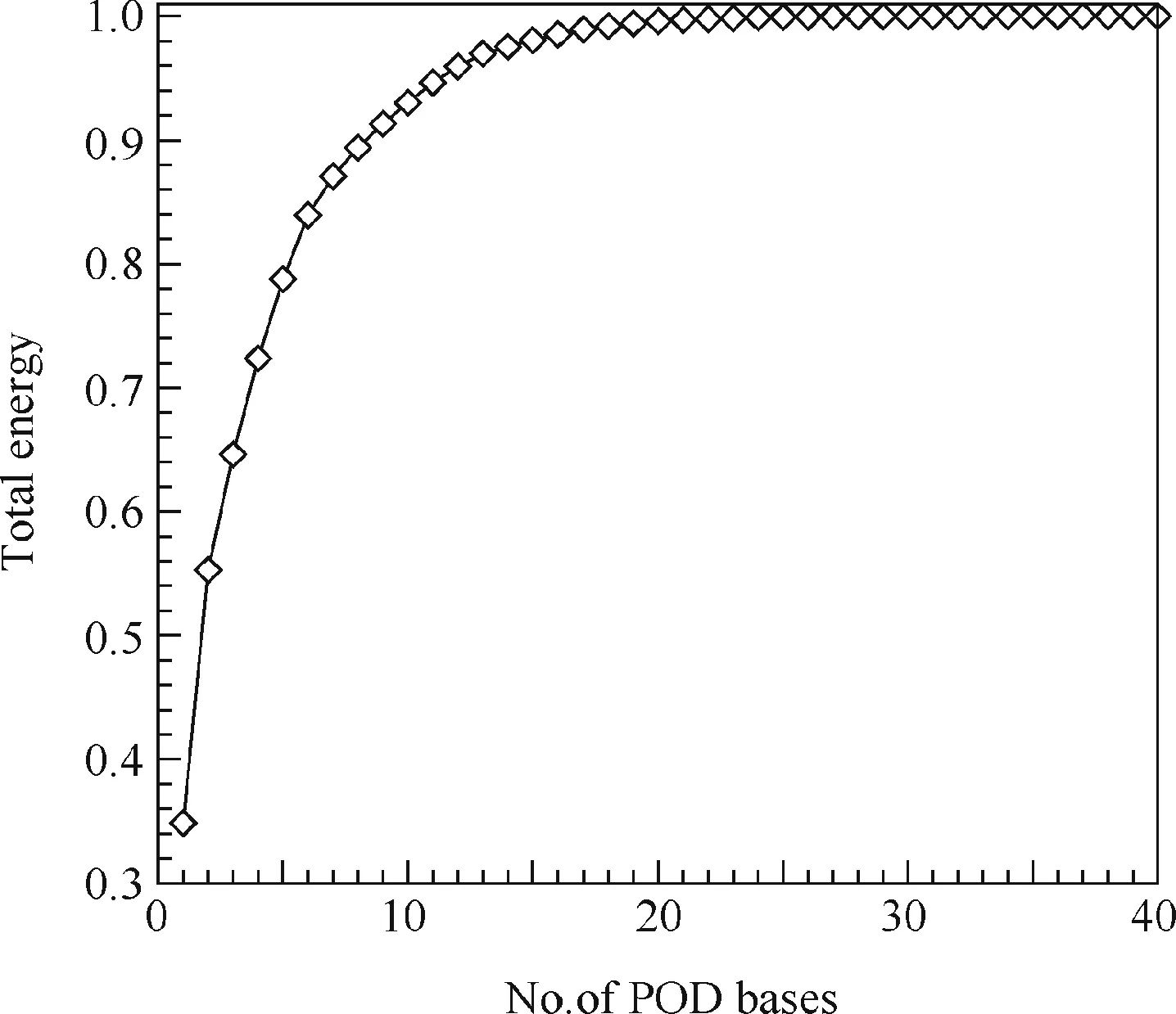
Fig.26 Total energy distribution of POD modes for ONERA M6 wing.

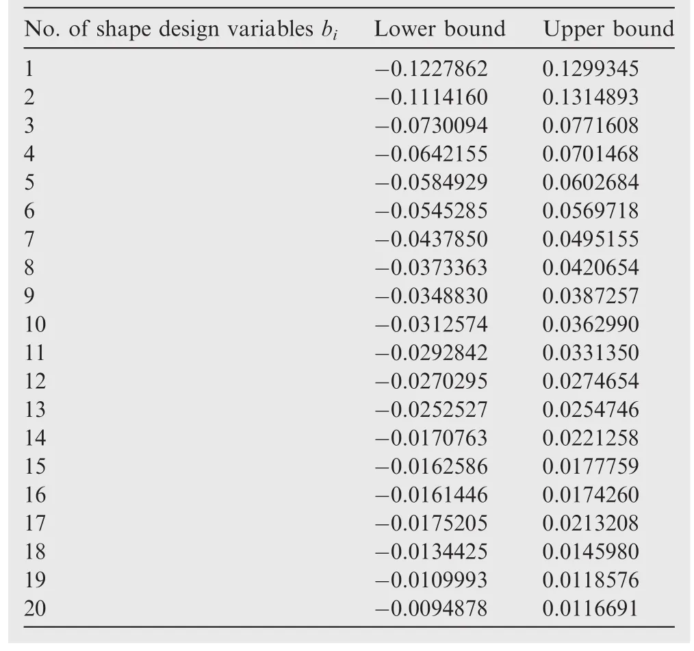
Table 6 New shape design variables for ONERA M6 wing optimization.

Fig.27 Comparison of surrogate model prediction and calculated results by full order CFD for ONERA M6 wing.

Fig.28 Convergence history for ONERA M6 wing optimization.

Table 7 Performance comparison for ONERA M6 wing optimization.

From the perspective of computational cost,the new optimization system improves the efficiency of conventional surrogate-based optimization significantly.Just as Table 5 shows,the total computational time for typical surrogate model is nearly 20 h and the majority of the computational time is spent in the flow solver for 600 training samples used in surrogate modeling.However,the new optimization system reduces the overall optimization time to just 6 h due to fewer design variables used in optimization,fewer training samples used for surrogate modeling and the acceleration method for samples calculation in surrogate modeling and optimization.Thus,the total computational time of new optimization system is only 1/3 of that of traditional SBO system.

4.3.Application to transonic wing

In order to examine the effectiveness and efficiency of the new optimization system on configurations with larger number of design variables,we further extend the aerodynamic optimization study to the three-dimensional aerodynamic design problem.Similar to the case of airfoil optimization problem,we also apply the typical surrogate-based optimization strategy for comparison.The ONERA M6 wing is chosen as the initial configuration.The CFD surface mesh is shown in Fig.24 and the mesh contains 6×105cells.

Fig.30 Comparison of shock waves.

Table 8 Computational cost summary for ONERA M6 wing optimization.

The objective is to minimize drag atMa=0.8395 andRe=18.14×106as maintaining a lift coefficientCL0=0.271537.In addition,the wing internal volume constraint is imposed.The optimization problem can be posed as follows:

Fig.29 Comparison of cross-section shapes and pressure coefficients.

We use FFD approach to parameterize the geometry in the typical SBO.Fig.25 shows the FFD volume and 66 FFD control points.As 8 control points on the leading and trailing edge of each span-wise station are fixed,the rest 42 control points are only permitted to vary inzdirection resulting in a total of 42 design variables.The bound of every design variable is[-0.01.0.01].

A set of 1000 samples used as snapshot ensemble for design space dimensionality reduction are generated in the original design space by LHS.According to Eq.(23),we can compute the covariant matrix C.The eigenvalues are arranged in descending order(λ1＞λ2＞λ3＞...＞ λ1000).As Fig.26 shows,the first 20 POD modes can capture 99.6%of the total energy of the original design space.Thus,we can take the POD basis coefficientsbiof the first 20 modes as new design variables and we manage to reduce the number of design variables from 42 to 20.

The wing aerodynamic shape in the low-dimensional space can be determined according to Eq.(25).Table 6 presents the upper and lower bounds for the new shape design variables,which are determined by the maximum and minimum modal coefficients of the original snapshot ensemble.

In order to reduce the computational cost,surrogate model is constructed.For the typical SBO,800 training samples are generated by LHS in the original design space and high fidelity full order CFD is evaluated at these points to create the training data set.On the other hand,600 training samples are obtained by LHS in the low-dimensional design space and all the training samples are evaluated by the acceleration approach mentioned in Section 3.3.After establishing the surrogate model,another 50 testing samples which serve as a model validation objective are obtained from both of the two design space.Just as Fig.27 shows,the average error between the predicted force coefficientCDand the results calculated by full order CFD is within 1 count.

Genetic algorithm is applied to handle the wing optimization problem.A population of 100 individuals and 100 generations are used while we have considered the following other parameters:probability of crossover=0.9 and probability of mutation=0.1. The convergence histories of typical surrogate-based optimization(denoted by FFD in the figure below)and new optimization system(denoted by POD in the figure below)are showed in Fig.28.The figure includes the result of every individual and the best of each generation which shows the new optimization system with fewer design variables converges much faster and converges to a better design.

Table 7 presents the optimization results.At the optimum,the lift coefficient is met and the new optimization strategy reduces the drag from 188.853 counts to 154.548 counts.The drag reduction is also larger than the typical SBO system.For a larger number of design variables,the benefits of reduction of DVs are more obvious.This can also be found in the case of Ackley’s function.In the limited generations and populations,it is harder for GA to converge in the original design space,let alone find a better solution.

The comparisons of surface pressure distribution and aerodynamic shapes at 3 different cross sections are showed in Fig.29.As can be seen from the sectionalCpcontours,the shock has been considerably weakened.From Fig.30,we can also see that the lambda shock wave is on the baseline while the shock has almost been erased after optimization.

Another crucial aspect is the computational cost,as shown in Table 8.The CFD simulation and optimization are carried out on a Windows server using Intel(R)Xeon(R)CPU E5-2620 v3@2.40 GHz,with a total of 2 nodes,12 cores per node.The total computational time for typical SBO is up to 240 h and the majority of the time is spent in the high-fidelity flow solver for 800 training samples used in surrogate modeling.On the other hand,it takes only 60 h for the new optimization strategy to accomplish the evaluation of 600 training samples through the acceleration method that we develop for samples calculation in surrogate modeling.

In summary,the computational cost of new optimization system constructed in our work is only 1/3 of that of traditional surrogate-based optimization system,thus significantly improving the efficiency of global optimization.

5.Conclusions

(1)A new optimization system is developed in this paper based on typical surrogate-based optimization framework and data dimensionality reduction method POD.The new optimization strategy includes dimensionality reduction of design space and acceleration approach for samples calculation in surrogate modeling.

(2)The optimizations of the transonic airfoil RAE2822 and the transonic wing ONERA M6 are performed using the new optimization system as well as traditional optimization system.In the airfoil case,we manage to reduce the number of design variables from 20 FFD control points to 10 POD coefficients which act as the new design variables for the optimization.In the wing case,the number of design variables is reduced from 42 to 20.Besides,the acceleration method for samples calculation in surrogate models allows a reasonable computational time while providing sufficient accuracy.The new design optimization system converges faster and it takes 1/3 of the total time of traditional optimization to converge to a better design,thus significantly reducing the overall optimization time and improving the efficiency of conventional global design optimization method.

Acknowledgement

This work was supported by the National Natural Science Foundation of China(No.11502211).

1.Jameson A.Aerodynamic design via control theory.J Sci Comput1988;3(3):233–60.

2.Kenway GKW,Martins JRRA.Multipoint aerodynamic shape optimization investigations of the common research model wing.AIAA J2015;54(1):113–28.

3.Zingg DW,Nemec M,Pulliam TH.A comparative evaluation of genetic and gradient-based algorithms applied to aerodynamic optimization.Eur J Comput Mech/Revue Europe´enne de Me´canique Nume´rique2008;17(1–2):103–26.

4.Painchaud Ouellet S,Tribes C,Tre´panier J,Pelletier D.Airfoil shaped optimization using a nonuniform rational B-spline parameterization under thickness constraint.AIAA J2006;44(10):2170–8.

5.Song W,Keane A.Surrogate-based aerodynamic shape optimization of a civil aircraft engine nacelle.AIAA J2007;45(10):2565–74.

6.Ghisu T,Parks GT,Jarrett JP.Accelerating design optimisation via principal components’analysis12th AIAA/ISSMO multidisciplinary analysis and optimization conference.Reston:AIAA;2008.

7.Ghoman SS,Wang Z,Chen PC.A POD-based reduced order design scheme for shape optimization of air vehicles.Reston:AIAA;2012.Report No.:AIAA-2012–1808.

8.Ghoman SS,Wang Z,Chen PC.Hybrid optimization framework with proper orthogonal decomposition based order reduction and design-space evolution scheme.J Aircraft2013;50(6):1776–86.

9.Toal DJ.Proper orthogonal decomposition&kriging strategies for design[dissertation].Southampton:University of Southampton;2009.

10.Toal DJ,Bressloff NW,Keane AJ.Geometric f i ltration using proper orthogonal decomposition for aerodynamic design optimization.AIAA J2010;48(5):916–28.

11.Zhao K,Gao ZH,Huang JT,Li Q.Aerodynamic optimization of rotor airfoil based on multi-layer hierarchical constraint method.Chin J Aeronaut2016;29(6):1541–52.

12.Viswanath A,Forrester AI,Keane AJ.Dimension reduction for aerodynamic design optimization.AIAA J2011;49(6):1256–66.

13.Lukaczyk T,Palacios F,Alonso JJ.Active subspaces for shape optimizationProceedings of the 10th AIAA multidisciplinary design optimization conference.Reston:AIAA;2014.p.1–18.

14.Qiu YS.Aerodynamic shape optimization methods based on data dimension reduction approaches[dissertation].Xi’an:Northwestern Polythchnical University;2014[Chinese].

15.Han Z,Zimmerman R,Görtz S.Alternative cokriging method for variable-f i delity surrogate modeling.AIAA J2012;50(5):1205–10.

16.Koziel S,Leifsson L.Surrogate-based aerodynamic shape optimization by variable-resolution models.AIAAJ2013;51(1):94–106.

17.Allaire D,Willcox K.Surrogate modeling for uncertainty assessment with application to aviation environmental system models.AIAA J2010;48(8):1791–803.

18.LeGresley PA,Alonso JJ.Dynamic domain decomposition and error correction for reduced order modelsAIAA 41st aerospace sciences meeting.Reston:AIAA;2003.

19.LeGresley PA.Application of proper orthogonal decomposition(POD)to design decomposition methods[dissertation].Stanford:Stanford University;2005.

20.LeGresley PA,Alonso JJ.Airfoil design optimization using reduced order models based on proper orthogonal decomposition.Proc AIAA Space2000;40(10):1954–60.

21.Bui-Thanh T,Damodaran M,Willcox K.Proper orthogonal decomposition extensions for parametric applications in compressible aerodynamicsProceedings of 21st AIAA applied aerodynamics conference.Reston:AIAA;2003.

22.Bui-Thanh T,Damodaran M,Willcox K.Aerodynamic data reconstruction and inverse design using proper orthogonal decomposition.AIAA J2004;42(8):1501–16.

23.Qiu YS,Bai JQ.Stationary flow fields prediction of variable physical domain based on proper orthogonal decomposition and kriging surrogate model.Chin J Aeronaut2015;28(1):44–56.

24.Sederberg TW,Parry SR.Freeform deformation of solid geometric models.Computer Graphics1986;22(4):151–60.

25.Zhu XX.The modeling technology of free curve and surface.Beijing:Science Press;2000.p.66–112[Chinese].

26.Singh JP.An improved Navier-Stokes flow computation of AGARD Case-10 flow over RAE2822 airfoil using Baldwin-Lomax model.Acta Mech2001;151(3–4):255–63.

27.Simpson TW,Mauery TM,Korte JJ.Kriging models for global approximation in simulation-based multidisciplinary design optimization.AIAA J2001;39(12):2233–41.

28.Holland JH.Genetic algorithms.Sci Am1992;267(1):66–72.

29.Liang YC,Lee HP,Lim SP,Lin WZ,Lee KH,Wu CG.Proper orthogonal decomposition and its applications-Part I:Theory.J Sound Vib2002;252(3):527–44.

30.Ly HV,Tran HT.Proper orthogonal decomposition for flow calculations and optimal control in a horizontal CVD reactor.Q Appl Math2002;60(4):631–56.

31.Jolliffe I.Principal component analysis.New York:John Wiley&Sons;2002.

32.Tang W,Wu J,Shi Z.identification of reduced-order model for an aeroelastic system from f l utter test data.Chin J Aeronaut2017;30(1):337–47.