A new remaining useful life estimation method for equipment subjected to intervention of imperfect maintenance activities

Changhua HU,Hong PEI,Zhaoqiang WANG,Xiaosheng SI,Zhengxin ZHANG

College of Science,High-Tech Institute of Xi’an,Shaanxi 710025,China

1.Introduction

With the increasing requirement for the safety and reliability of engineering equipment,Prognostics and Health Management(PHM)technique has received widespread attention in the academic and industrial field during the past decades.1–3As the key part of PHM,Remaining Useful Life(RUL)estimation can be used to determine the maintenance time,inspection interval,or spare parts’ordering quantity by minimizing economic cost or mitigating failure risk,2–7and hence,increasing attention has been paid to the RUL estimation domain.The remaining useful life of an asset is generally defined as the length from the current time to the end of the useful life.2The existing RUL estimation studies can be grouped into the following two types:physics-based methods and data-driven methods.1For these two types of methods,physics-based methods are based on the identification of potential failure mechanisms for a device,product,or system,and thus the failure can be easily located and insulated.However,due to the complexity of the engineering system as well as the diversity and uncertainty of the operating environment,it is extremely difficult to identify the potential failure mechanisms.Owing to the rapid development of sensory technology,data-driven methods have become the mainstream in the current RUL estimation domain.

The commonly-used data-driven methods include Wiener process,Gamma process,and Markov chain.2Because Wiener process can be adopted to describe both the monotonous and non-monotonous degradation processes,it exhibits better performance compared with Gamma process and Markov chain in many engineering practice including rotating element bearings,self-regulating heating cables,laser generator and bridge beams.Therefore,Wiener process based degradation models have been studied intensively in literature.Based on Wiener process with a linear drift,Tseng et al.determined the lifetime of the light intensity of LED lamps in Ref.8.Ye et al.investigated linear-drifted Wiener process with measurement error and developed a mixed effects model motivated by the degradation process of magnetic heads used in hard disk drives.9Due to the extensive existence of the nonlinear degradation patterns,a nonlinear-drifted Wiener process model as well as an analytical RUL distribution derivation method was presented in Ref.10.Wang et al.further proposed an additive Wiener process based RUL estimation method for the hybrid deteriorating systems,where the stochastic dependencies between different deteriorating patterns were considered.11Based on Wiener process with a nonlinear drift,Huang et al.presented a recursive filter algorithm,which could improve the estimation accuracy of the RUL.12Recently,a nonlineardrifted Wiener process modeling method was proposed for the RUL estimation of rechargeable batteries by taking multiple hidden states into consideration.13

Most of the existing RUL studies assumed that the degrading equipment was not maintained during its life cycle.4–14Nevertheless,in practice,when the degradation level of the equipment exceeds a specified threshold,maintenance activities are often carried out for the equipment to improve the performance.According to the effect of maintenance,maintenance activities can be divided into perfect maintenance,imperfect maintenance,and minimal maintenance.15Specifically,perfect maintenance can restore the equipment to an as-good-as new state,and minimal maintenance can restore the equipment to an as-bad-as old state.Differently,imperfect maintenance can restore the equipment to the state between as good as new and as bad as old.16–23Therefore,compared with perfect maintenance and minimal maintenance,imperfect maintenance is more general in the engineering practice,examples of imperfect maintenance are spraying lubricant for drill bit,adjusting the dynamic balance of the fan.21–23Imperfect maintenance activities can normally slow down the degradation of the equipment,thereby prolonging the life of the equipment.15If the influence of the imperfect maintenance is not well taken into account,the RUL estimation for the equipment subjected to the intervention of imperfect maintenance activities may have large biases.Thus,imperfect maintenance activities have a critical influence on the RUL estimation of such degrading equipment,and it is important to account for the influence of the imperfect maintenance activities when we estimate the RUL of the equipment in such situations.21–23

However,although imperfect maintenance has attracted great attention in maintenance activities scheduling area,24–26few studies could be found in literature to consider the influence of imperfect maintenance activities on RUL estimation.You and Meng proposed an extended proportional hazards model to carry on the simulation analysis for the maintenance activities,27which could obtain the mean and variance of the RUL,but could not obtain the distribution of the RUL.Wang et al.used Wiener process with negative jumps to estimate the RUL of the equipment subjected to imperfect maintenance activities,22which only considered the influence of maintenance activities on the degradation level but ignored the influence of maintenance activities on the degradation rate.Contrarily,Zhang et al. estimated theRUL of the equipment under the considerationof influence of maintenance activities on the degradationrate, but ignored the influence of maintenance activities onthe degradation level.23In the engineering practice, it is well recognizedthat imperfect maintenance activities have a certaininfluence on both the degradation level and the degradationrate.21,23,28For example, as a commonly-used imperfect maintenancestrategy, welding process for metal component can reducethe crack length, but it can also destroy the physical mechanismof inner materials and therefore accelerate the degradation rateof the metal component. It should be noted that, although newproducts also have heterogeneous phenomenon and differentdegradation rates,9–11this is different with what we will consider in this manuscript in that the degradation rate is assumed to become larger after maintenance.In order to appropriately characterize the influence of the imperfect maintenance activities and accurately estimate the RUL of the equipment,these two factors should be taken into account at the same time.

Aimed at the aforementioned problem in current RUL estimation studies of the degrading equipment subjected to imperfect maintenance activities,this paper proposes anew degradation modeling and RUL estimation method considering the influence of imperfect maintenance activities on both the degradation level and the degradation rate.Compared with the similar studies in literature(such as Wanget al.22and Zhang et al.23),the main contributions of this paper are twofold:(1)considering the influence of imperfect maintenance activities on both the degradation level and the degradation rate;(2)deriving the Probability Density Function(PDF)of the RUL for the equipment subjected to imperfect maintenance by the convolution operator.Specifically,a stochastic degradation model considering the influence of imperfect maintenance activities is firstly constructed based on the diffusion process.Based on the constructed model,the PDF of the RUL is derived by the convolution operator under the concept of First Hitting Time(FHT).To implement the presented method,the unknown model parameters are estimated by the maximum likelihood estimation method and Bayesian method based on the available Condition Monitoring(CM)data and maintenance data.The results of a simulated example and a practical case are provided to demonstrate the superiority of the proposed method.

The remainder of the paper is organized as follows.Section 2 gives the problem description and associated assumptions.Section 3 presents the degradation modeling method based on the diffusion process and derives the PDF of the RUL.The parameter estimation process is given in Section 4.A numerical example is provided in Section 5 for demonstration.Section 6 provides a practical case study for illustration.The main conclusions are summarized in Section 7.

2.Problem description and assumptions

2.1.Problem description

For the engineering equipment,the degradation level can be obtained by CM technique,and it is compared with the Preventive Maintenance(PM)threshold to make the maintenance decisions.When the degradation level exceeds the preset PM threshold,the maintenance activities will be carried out.Considering the effectiveness of PM,we can further classify the PM as perfect maintenance,minimal maintenance and imperfect maintenance.As mentioned above,due to the generalization of imperfect maintenance activity relatively to the other two PM strategies,we will focus on this kind of maintenance scheme in this paper.Specifically,the imperfect maintenance activities can not only reduce the degradation level of the system,but also increase the system’s degradation rate.In order to ensure the operating reliability and lower the maintenance cost,the upper limit of the total number of maintenance activities is assumed to be finite,denoted as n.In other words,when the number of the imperfect maintenance reaches the specified n,the engineering equipment will no longer be maintained,and it will be totally replaced before its degradation level first hits the specified failure threshold.

Fig.1 provides a schematic diagram of the degradation trajectory considered in this paper,which characterizes the continuous degradation process of the engineering equipment subjected to the intervention of imperfect maintenance activities.In Fig.1,the PM threshold of the equipment is denoted by ωpand the failure threshold is denoted by ω.Ti（i≤ n，i∈ N+）denotes the time of the ith maintenance,and Tn+1denotes the failure time.We use ti，jto represent the CM time,where i is the maintenance number before ti，j,j（j∈ ［0，ri］）is the CM number after the ith maintenance,and riis the total CM number between Tiand Ti+1.It can be readily found that the time instant denoted by ti-1，ri-1，Ti，and ti，0is equal to each other,i.e.,ti-1，ri-1=Ti=ti，0.

As shown in Fig.1,the degradation process can be divided into n+1 stages during the whole life cycle by the total number n of imperfect maintenance activities, i.e.,（0，T1），（T1，T2），···，（Tn，Tn+1）.We assume that every stage of the degradation process is independent with each other.It can be intuitively seen that the life T of the equipment subjected to the intervention of imperfect maintenance activities can be regarded as the sum of the operating time of each stage,i.e.,T=∑where Rirepresents the operating time of the（i+1）th stage.

Based on the above description,we will study the following problems in this paper:

(1)How to construct the degradation model of the equipment subjected to the intervention of imperfect maintenance activities;

(2)How to derive the PDF of the RUL at any time for the equipment subjected to the intervention of imperfect maintenance activities;

(3)How to estimate the parameters in the degradation model based on the CM data and the maintenance data.

2.2.Assumptions

On the basis of the problem described above,we propose the assumptions required either for practical consideration,or for modeling simplification.

Fig.1 Degradation trajectory under intervention of maintenance activities.

(1)The equipment is monitored perfectly and periodically.

(2)The PM is imperfect and can restore the health condition of the equipment to a state between as good as new and as bad as old.

(3)The total number of the PM is finite.Specifically,when the maintenance number for the equipment reaches the specified upper limit n,the PM activities will not be carried out any longer due to the reliability and cost considerations.

(4)If the degradation level is between the PM threshold ωpand the failure threshold ω,a PM is carried out immediately.

(5)If the degradation level exceeds the failure threshold ω,the equipment is required to be replaced immediately.

(6)If the degradation level is less than the PM threshold,the equipment is left unchanged until the next CM time.

Assumption 1 is common in degradation modeling practice.2,3,11Assumption 2 is due to the consideration for the engineering practice and is widely accepted in the academic field.15–17It is noted that assumptions 3–6 have been widely adopted in maintenance and inventory modeling practices for modeling simplification(see for examples in Refs.21,23,28).

3.Degradation modeling and RUL estimation

3.1.Degradation modeling

In this paper,diffusion process is utilized to describe the nonlinear stochastic degradation under the intervention of imperfect maintenance activities,i.e.,the degradation path of the equipment can be modeled by diffusion process at each stage between two successive maintenances.The degradation level after the ith maintenance activity can be denoted as

where X（t）is the degradation level at time t;i（i≤ n，i∈ N+）is the maintenance number performed before t;ηiis the residual degradation coefficient after the ith maintenance activity,which is assumed to follow a normal distribution,i.e.,ηi～ N（1-exp（-ai），b）,and a and b are hyperparameters29;ωprepresents the PM threshold of the equipment specified by industrial standard and expert experience; μ（τ，θ）is used to characterize the nonlinear stochastic nature,τ is the integral variable,and θ is the fixed parameter related to the degradation rate;λiis a random parameter related to the degradation rate.From the mathematical point,the degradation rate can be regarded as the derivative of the degradation level.To describe the influence of maintenance activities on the degradation rate,we introduce the degradation rate changing factor cias the maintenance parameter and assume that λiis formulated as λi=ciλ0,where λ0denotes the fixed parameter related to the degradation rate,and ciis the degradation rate changing factor after the ith maintenance activity.The PDF of ciis denoted by f（ci|i，Υ）,where Υ is the parameter vector in the distribution of ci.In particular,c0=1.Tiis the time of the ith maintenance,σBis the diffusion coefficient,and B（·）is the standard Brownian Motion(BM).

Remark 1.The reasons that the residual degradation coefficient is assumed to follow the specified normal distribution are twofold.First,it is easier to obtain the analytical results or it can facilitate the derivation process under the normal distribution,which is desirable from both the theoretical and practical angles.Second,it is noted that the normal distribution has plenty of good characteristics,whose mean and variance for the residual degradation coefficient had been given to describe imperfect maintenance model in Ref.29.

Remark 2.The reason that the degradation rate changing factor ciafter the ith maintenance activity is used to describe the influence of imperfect maintenance activities on the degradation rate is mainly to facilitate derivation,which is modeled by Zhang et al.23

3.2.Derivation of PDF of RUL

Now,we discuss how to estimate the RUL for the degrading equipment defined in Eq.(1).Based on the concept of FHT,the RUL at time ti，jis defined as10,11

where Li，jis the RUL at time ti，jwith its realization li，j,and xi，jis the degradation level at time ti，j.

Based on the analysis in Section 2,the degradation process can be divided into n+1 stages.In order to illustrate the RUL intuitively and derive the PDF of the RUL theoretically,we need to define the following variables: Ln，j=inf｛ln，j:denotes the RUL at time t,R=n，ji，jdenotes the remaining operating time at time ti，jfor the （i+1）th stage,Ri+k=denotes the operating time of the （i+k+1）th stage, anddenotes the operating time of the （n+1）th stage.Thus,as shown in Fig.2,the RUL Li，jat time ti，jcan be represented as

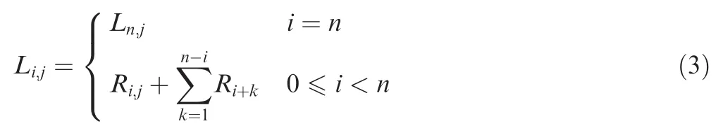
According to Eq.(3)and Fig.2,the RUL estimation for the equipment subjected to the intervention of imperfect maintenance activities can be divided into two cases,i.e.,i=n and 0≤i＜n.We will derive the PDF of the RUL for the equipment in the following section.

Based on the work by Gnedenko and Kolmogorov,30the PDF of the RUL can be further denoted by

where fLi，j（li，j）is the RUL at time ti，j,fLn，j（ln，j）is the RUL at time tn，j,fRi，j（ri，j）is the PDF of the remaining operating time for the （i+1）th stage,fRi+k（ri+k）is the PDF of the operating time for the （i+k+1）th stage,fRn（rn）is the PDF of the operating time for the （n+1）th stage,and ⊗ is the symbol of convolution operator.

In order to derive the PDF of the RUL,it is necessary to obtain the PDFs of the defined variables above.We assume that the degradation rate changing factor cifollows a normal distribution for simplification,i.e.,ci～ N（iμc，σ2c）,where the parameters in the distribution is denoted by Υ = （μc，σ2c）,and obviously,the mean of stochastic parameter ciis growing with the increase of the maintenance number i.

Based on the above analysis,the PDF of the RUL can be theoretically derived for these two cases.

Case 1.When i=n,according to the RUL described in Eq.(3),we can derive the conditional PDF of the RUL at time tn，jon condition that the stochastic parameter cnis given by the method proposed in Ref.10:

Considering the stochastic nature of the parameter cn,the unconditional PDF of the RUL can be analytically derived based on the law of total probability.To facilitate the derivation process,the following lemma should be provided.

Lemma 110.If Z ～ N（μ，σ2）,and ω1，ω2，A，B ∈ R,C ∈ R+,then

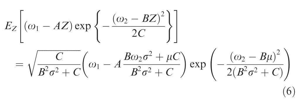
The proof of Lemma 1 can be deduced by generalizing the result in Ref.10,and thus it is omitted here.Based on the above lemma,we can obtain the analytical PDF of the RUL at time tn，j.

Proposition 1.For the stochastic degradation process defined in Eq.(1),based on the concept of the FHT,the analytical PDF of the RUL at time tn，jcan be obtained by

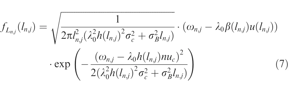
Fig.2 Relationship between RUL and defined variables.

Proof.Based on the law of total probability,the PDF of the RUL at time tn，jcan be written as

where Ωnis the parameter space of cn,f（cn）is the PDF of cn,and fLn，j（ln，j|cn）is the conditional PDF of the RUL at time tn，j.

Substituting Eq.(5)into Eq.(8),we have

Eq.(7)can be readily obtained based on Eqs.(6)and(9).

This completes the proof of Proposition 1.

Case 2.When 0≤i＜n,according to the PDF of the RUL defined in Eq.(4),to derive the PDF of the RUL,it is necessary to derive the PDF fRi，j（ri，j）of the remaining operating time for the （i+1）th stage,the PDF fRi+k（ri+k）of the operating time for the （i+k+1）th stage,and the PDF fRn（rn）of the operating time for the （n+1）th stage.The proposition is given as follows to obtain the PDF fRi，j（ri，j）,and the conditional PDFs

Proposition 2.For the stochastic degradation process defined in Eq.(1),based on the concept of the FHT,we have the following results:

(1)The PDF fRi，j（ri，j）of the remaining operating time for the（i+1）th stage can be denoted by

(3)The conditional PDF fRn（rn|ηn）of the operating time for the （n+1）th stage can be denoted by

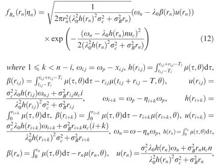
ηi+kdenotes the residual degradation coefficient after the（i+k）th maintenance activity,and ηndenotes the residual degradation coefficient after the nth maintenance activity.

The proof process is similar to the proof of Proposition 1,and hence we omit it here.

Due to the stochastic characteristics of ηi+kand ηnin the corresponding PDFs,Eqs.(11)and(12)denote the conditional PDFs,which have difference with Eq.(10).Hence,we can utilize the law of total probability to derive the PDFsandOwing to the fact that the conditionaland fRn（rn|ηn）are too complex to derive the theoretical expressions,the Monte-Carlo(MC)algorithm is adopted to calculate the PDFs fRi+k（ri+k）and fRn（rn）.

Based on Proposition 1,Proposition 2 and Eq.(4),we can obtain the PDF of the RUL for the equipment.The following lemma should be provided as the basis.

Lemma 231.If Y1，Y2，···，Ynare the independent random variables with the corresponding PDFs fY1（y1），fY2（y2），···，fYn（yn）,then the PDF of the random variablecan be denoted by

where fYiis one of the PDFs fY1（y1），fY2（y2），···，fYn（yn）.

The proof of Lemma 1 can be deduced by generalizing the result in Ref.31,and thus it is omitted here.Furthermore,based on the Lemma 2,the PDF of the RUL of the equipment can be denoted by

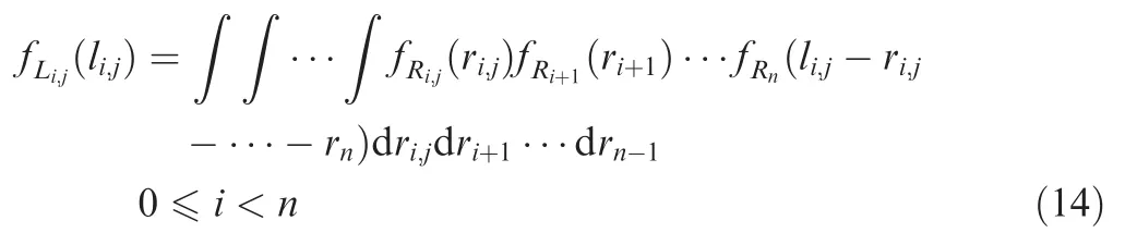
Substituting the expressions of the PDFs fRi，j（ri，j）,fRi+k（ri+k）（1 ≤ k ＜ n-i）,and fRn（rn）into Eq.(14),we can obtain the PDF of the RUL of the equipment.The calculation of Eq.(14)involves multiple integral operations,which is so complicated that we cannot obtain the analytical expression.To obtain the PDF of RUL,a numerical simulation algorithm is formulated in this paper to calculate the PDF of the RUL.Specifically,MC simulation algorithm is also used to calculate the PDF f（li，j）of the RUL at any time ti，j（0 ≤ i＜ n）as follows.

Step 1.If 0 ≤ i＜ n,we can obtain the PDFs fRi，j（ri，j）,andbased on Eqs.(10)–(12)respectively.

Step 2.Select a sufficiently large positive integer(denoted by M1),we can sample from the PDFs f（ηi+k）and f（ηn）of residual degradation coefficient respectively.The pth specific sampling values are denoted by0 ≤ p ≤ M1.The PDFs fRi+k（ri+k）and fRn（rn）can be written as

Step 3.Select a sufficiently large positive integer(denoted by M2)again and simulate the realizations from the PDFs fRi，j（ri，j）,fRi+k（ri+k）（1 ≤ k ＜ n-i）.We denote the pth speciif c realization bywhere 0 ≤ p ≤ M2.

Step 4.For the sufficiently large number M2,based on the law of large numbers,we can approximately obtain the PDF fLi，j（li，j）of the RUL at any time ti，j:

In order to have a better understanding of the MC simulation algorithm,a flowchart of the MC simulation algorithm is provided in Fig.3.

4.Parameter estimation

The parameters that are needed to be estimated include the following three parts:residual degradation coefficient,degradation parameters and maintenance parameters.

4.1.Residual degradation coefficient estimation

The residual degradation coefficient can be estimated through the Maximum Likelihood Estimation(MLE)method.32,33It is assumed that there are m groups of historical equipment which are independent for each other.Letdenote the residual degradation data of the sth（1 ≤ s≤ m，s∈ N+）historical equipment after each activity,whereand s is the number of the sth historical equipment.According to the degradation process defined in Eq.(1),the relation between the residual degradation coefficient and the residual degradation of the sth equipment at the ith PM activity can be given by

Based on Eq.(18)and the residual degradation of the sth equipment after each activity,we can obtain the residual degradation coefficientof the sth equipment after each PM activity,whereFrom Eq.(1),we can find that the parameters in the distribution of the residual degradation coefficient ηiinclude a and b.The estimation of the parameters a and b is realized by the MLE.The loglikelihood function ℓ（a，b）is given by

Fig.3 Flowchart of proposed MC simulation algorithm.

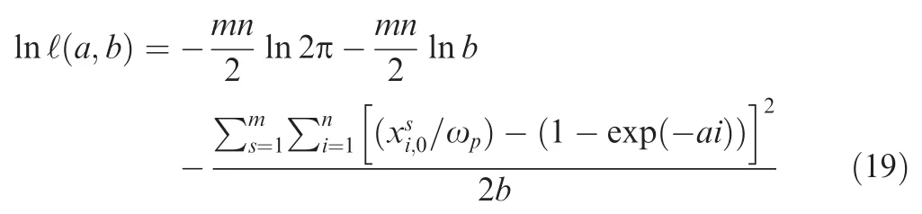
In order to maximize the log-likelihood function in Eq.(19),we take the partial derivative of lnℓ（a，b）with respect tob:

Let the partial derivative equal zero,and we have

The log-likelihood function lnℓ（a）can be deduced by taking Eq.(21)into the log-likelihood function Eq.(19).By maximizing lnℓ（a）,we can obtain the MLE of parametera.Further,the estimation ofbcan be obtained by substituting the estimation ofainto Eq.(21).

4.2.Degradation parameters estimation

The degradation parameters are also estimated utilizingmgroups of historical degradation data.We suppose that all the observed degradation data of thesth historical equipment is denoted byBased on the above assumptions,the degradation changing factorc0for the first stage equals one,while the degradation changing factorcifor the （i+1）th stage follows a normal distribution,i.e.,In order to make full use ofmgroups of historical degradation data,we should analyze each stage respectively.

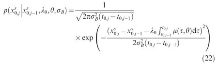
For the first stage,based on Eq.(1)and the basic properties of the diffusion process,we have

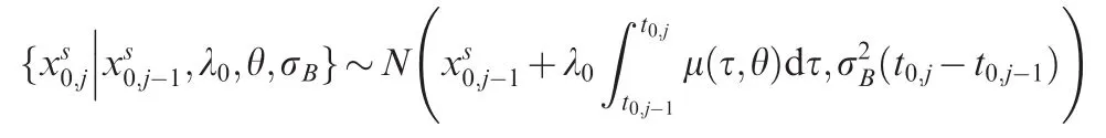
and hence,the conditional PDF ofcan be written as

According to the Bayesian chain principle and the Markov property of the diffusion process,we have

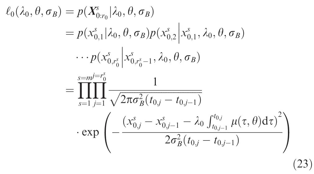
where ℓ0（λ0，θ，σB）denotes the likelihood function for the first stage.

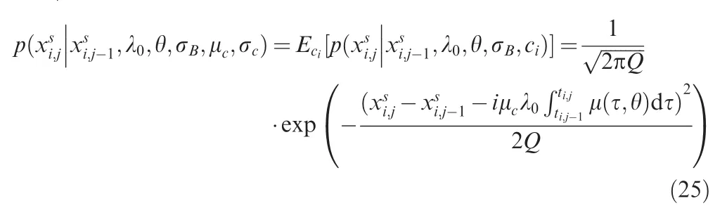
Similarly,for the （i+1）th stage,the conditional PDF ofcan be written as

Owing to the unknown characteristics ofci,it is difficult to employ MLE to estimate the degradation parameters.According to Lemma 1, the conditional PDF ofcan be given by

Owing to the assumption that every stage of the degradation process is independent with each other,the likelihood function ℓ（λ0，θ，σB，μc，σc）based onmgroups of historical degradation data can be written as

The MLE values of （λ0，θ，σ2B，μc，σc）can be obtained by maximizing Eq.(27).It is worth noting that the MLE values of（μc，σc）can be used as the prior distribution of maintenance parameters.

4.3.Maintenance parameters estimation

We suppose that the observed degradation data of the operating equipment between the time of thekth PM and the timetk，rkare denoted aswherekis the PM number of the operating equipment before the timetk，rk,andrkis the CM number of the operating equipment after thekth PM.The following proposition is given to estimate the maintenance parameters

Proposition 3.The posterior estimates of the maintenance parameters）at tk，rkcan be written as

Proof.Based on the degradation model described in Eq.(1)and the basic characteristic of the diffusion process,we have

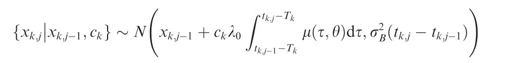
By employing the Bayesian chain principle,we can obtain the joint probability density ofconditional on the stochastic parameter ck:

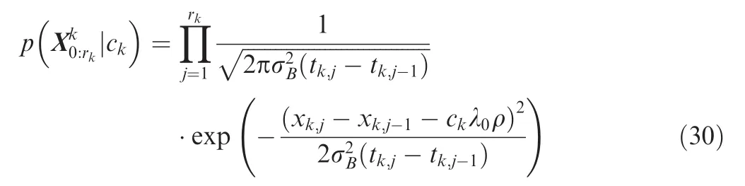
Let the prior distribution of ckbe denoted by p（ck）,whose mean and variance are kμc，k0andrespectively.can be obtained based on the degradation data before the kth PM.

According to Bayesian theorem,the posterior distribution of the stochastic parameter ckcan be given by

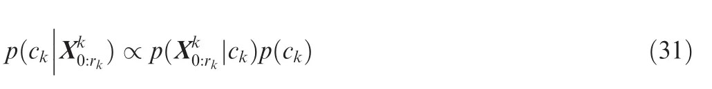
This completes the proof.□

The main procedure of the aforementioned parameter estimation process can be summarized as follows.

(1)The parameters （a，b）are estimated by the MLE based on the observed residual degradation data of the historical equipment after each PM;

(3)The posterior parameters ofare updated based on the real-time obtained degradation databy Eqs.(28)and(29),where the priors ofcan be obtained based on the observed degradation data of the historical equipment.

In order to have an intuitive understanding of the parameter estimation and RUL estimation method,we provide a flowchart of the RUL estimation method proposed in the paper,as shown in Fig.4.

Fig.4 Flowchart of proposed RUL estimation method.

Table 1 Parameter setting.

5.Numerical example

This section verifies the effectiveness of the RUL estimating method proposed in the paper by a numerical example.

5.1.Data generation via simulation

In order to generate the simulated data,it is necessary to specify the parameters in Eq.(1).We set the parameters in Table 1 and select μ（τ，θ）= θτθ-1for simplification as used in the Ref.10.Furthermore,we set the sampling time interval Δt=0.05.

After setting the parameters,we generate three simulation degradation trajectories according to the degradation model defined in Eq.(1).The simulation degradation trajectories along with the PM threshold and the failure threshold are illustrated in Fig.5.The simulation trajectories 1 and 2 as the historical equipment are used to estimate the residual degradation coefficient and the degradation parameters of the model defined in Eq.(1).The simulation trajectory 3 is used to update the maintenance parameters and estimate the RUL of the degradation process in real time.

5.2.Results and comparison

Fig.5 Three simulation degradation trajectories.

We can obtain the residual degradation after each maintenance for the simulation trajectories 1 and 2, i.e.,Therefore,the residual degradation coefficient of the simulation trajectories 1 and 2 after each maintenance activity can be derived based on Eq.(18),i.e.,and.Table 2 provides the calculated residual degradation coefficient after each PM for the simulation trajectories 1 and 2.

Therefore,the MLE value of a can be determined by taking the residual degradation coefficient into the log-likelihood function lnL（a）.The estimated values of a and b are^a=0.2016,and^b=0.0013.

According to Section 4.2,we can obtain the MLE values of the degradation parameters）based on the simulation trajectories 1 and 2,as shown in Table 3.From Table 3,we canfind that the estimation values for the degradation parameters have little difference with the true values,which verifies the effectiveness of the proposed degradation parameter estimation method.

Based on Proposition 3,the distribution parameters（μ）can be updated online utilizing the degradation data of the simulation trajectory 3.The initial value （）can be selected according to the degradation data of the historical equipment.Figs.6 and 7 illustrate the updated results.FromFigs.6 and 7,we can find that the deviations between the initial values of（）and their true values are large at the early stage because the historical sample is too few to characterize the truth of the parameters.However,with the acquisition of the degradation data,the estimation values of μcand σcare gradually approaching the true values,which verifies the effectiveness of the proposed maintenance parameter updating method.

Table 3 Degradation parameter estimation.

Fig.6 Updated results of μc.

Table 2 Residual degradation coefficient for simulation trajectories 1 and 2.

Fig.7 Updated results of σc.

After obtaining the estimated parameters,we select ti，j=7 and ti，j=11 as the time for RUL estimation.From the simulation trajectory 3,we can find that the first PM occurs at 6.95 and the second PM occurs at 10.95.Therefore,when ti，j=7,there exists one PM activity before ti，j,i.e.,i=1,and there exists one CM datum after the first PM,i.e.,j=1.When ti，j=11,there exist two PM activities before ti，j,i.e.,i=2,and there exists one CM datum after the second maintenance,i.e.,j=1.Based on Proposition 2,the PDF fRi，j（ri，j）of the remaining operating time for the （i+1）th stage,the PDF fRi+k（ri+k）of the operating time for the （i+k+1）th stage,and the PDF fRn（rn）of the operating time for the （n+1）th stage can be derived. After obtaining the PDFs fRi，j（ri，j） and fRi+k（ri+k）（1 ≤ k ＜ n-i）,we can sample from the PDFs by the MC sampler.It is worth mentioning that the calculation time of the MC simulation algorithm at ti，j=7 and ti，j=11 is 45.96 s and 38.35 s respectively.In order to verify the effectiveness of the RUL estimation method proposed in the paper,the method that considers the influence of imperfect maintenance activities on both the degradation level and the degradation rate(i.e.,the method proposed in this paper)is denoted by M1,the method ignoring the influence of imperfect maintenance activities on the degradation rate is denoted by M2(i.e.,the method proposed in Ref.22),while the method ignoring the influence of imperfect maintenance activities on the degradation level is denoted by M3(i.e.,the method proposed in Ref.23).Figs.8 and 9 provide the PDFs of the RULs for the equipment at time 7 and time 11 for these three methods.

Fig.8 PDF of RUL at ti，j=7 for three methods.

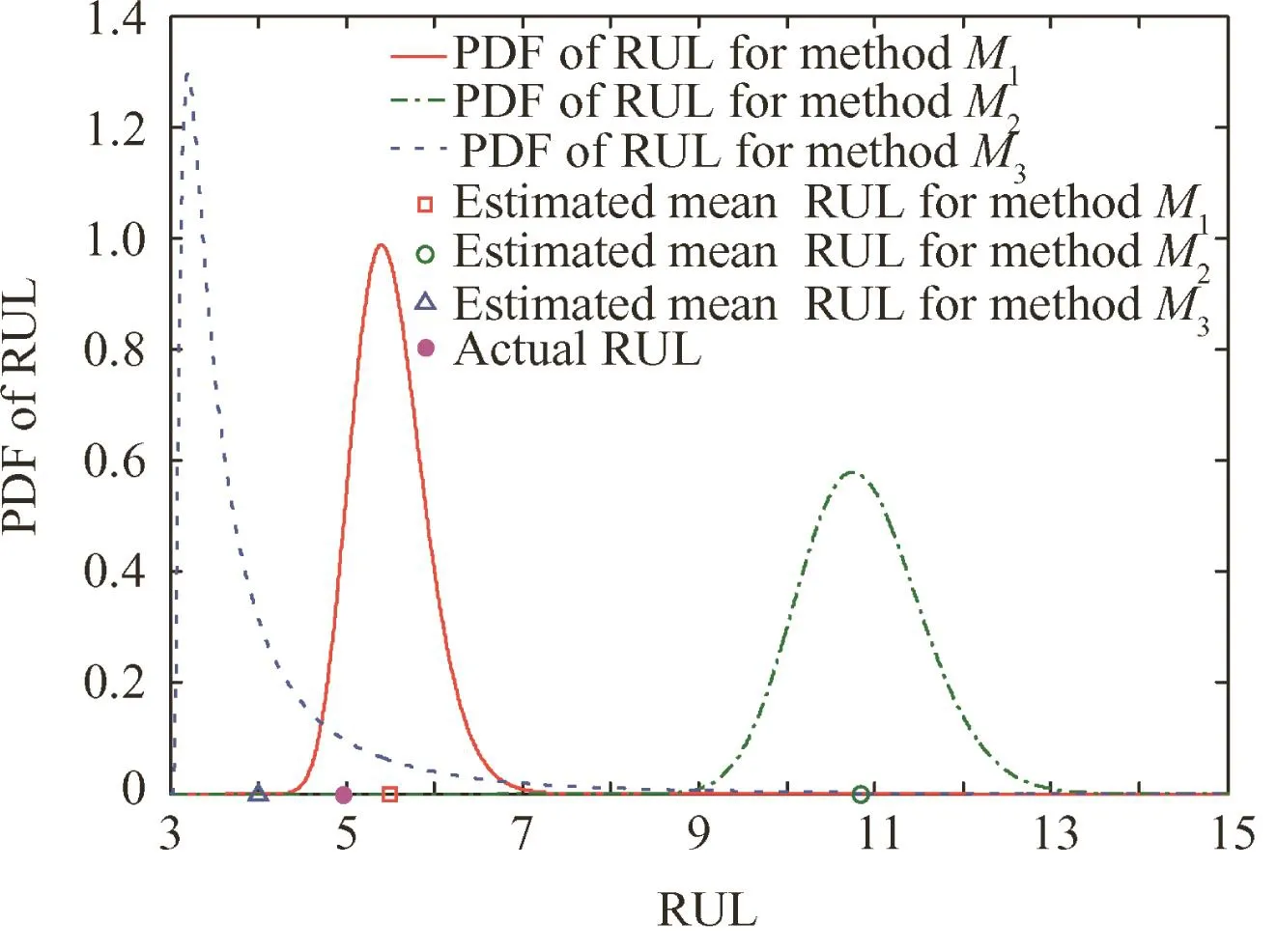
Fig.9 PDF of RUL at ti，j=11 for three methods.

According to the above analysis,when ti，j=7,we can sample from the PDFs f（r1，1）,f（r2）,and f（r3）.After we obtain the sampling results,the PDF of the RUL can be approximately calculated by Eq.(17),which is illustrated in Fig.8.From Fig.8,we can find that the estimated RUL by method M1is more accurate than that by the other two methods M2and M3.The estimated mean RULs for methods M1,M2,and M3are 10.0,16.8,and 6.2 respectively,while the actual RUL is 8.9.So,method M2overestimates the RUL of the equipment,and the method M3underestimates the RUL of the equipment.Because methods M2and M3ignore the double influence of imperfect maintenance on the degradation level and the degradation rate.We can also find that the deviation between the estimated mean RUL for method M1and the actual RUL seems to be a bit large.This is because the degradation data obtained at ti，j=7 is too limited,which leads to the uncertainty of the maintenance parameter estimation.

Similarly,when ti，j=11,we can sample from the PDFs f（r2，1）and f（r3）.Based on the sampling results,the PDF of RUL can be approximately calculated by Eq.(17),as illustrated in Fig.9.From Fig.9,the estimated mean RULs for methods M1,M2,and M3are respectively 5.4,10.8,and 4.0,while the actual RUL is 4.9.Obviously,the estimated mean RUL by method M1is more accurate than the estimated mean RULs by methods M2and M3.Owing to the fact that the CM data obtained at ti，j=11 are increasing,the deviation between the estimated mean RUL by method M1and the actual RUL is gradually decreasing.However,the PDF of the RUL is calculated approximately by Eq.(17),and hence,there still exists a certain deviation between the estimated mean RUL of method M1and the actual RUL.

We have considered the situation of 0≤ i＜ n above.In the following part,we will further consider the situation of i=n.Specifically,we select a series of time instants for RUL estima-tion,i.e.,｛14.5，14.6，14.7，14.8，14.9，15.0，15.1，15.2，15.3，15.4，15.5｝.Owing to the fact that the influence of imperfect maintenance activities on the degradation level can be re flected by the degradation data,the method that ignores the influence of imperfect maintenance activities on the degradation level(i.e.,method M3)will be obviously inappropriate for the RUL estimation here,and hence,this method is not employed for comparison.Fig.10 provides the estimated PDFs and means of the RULs at the chosen estimation times for methods M1and M2.

From Fig.10,we can find that the estimated mean RUL by method M1is close to the actual RUL,while the estimated mean RUL for method M2seriously deviates from the actual RUL.The main reason is that method M2ignores the influence of the imperfect maintenance activities on the system’s degradation rate.Therefore,when method M2is used,it will overestimate the RUL of the equipment,which may lead to catastrophic accidents for the engineering equipment in practice.

To further compare the RUL estimation accuracy between these two RUL estimation methods quantitatively,the Mean Squared Error(MSE)for the RUL estimation is adopted,which is defined as11

Based on Eq.(33),we can obtain the MSE at each estimation time for these two methods,which is shown in Fig.11.We can see clearly from Fig.11 that the MSE of the RUL estimation by method M1is far less than the MSE of the RUL estimation by method M2.As a result,the double influence of imperfect maintenance activities on degradation level and degradation rate should be taken into consideration while modeling the degradation and estimating the RUL of the equipment subjected to the intervention of imperfect maintenance activities.

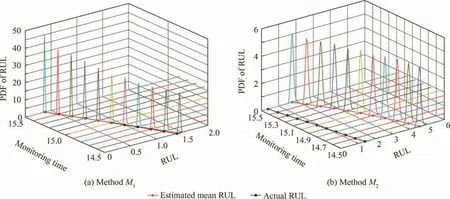
Fig.10 Estimated PDFs and means of RULs of the gyro by method M1and M2.

Fig.11 MSE of estimated RULs at chosen times.

6.Practical case study

This section provides a practical case study of gyroscopes(abbreviated as gyros in this paper)in the inertial navigation systems to demonstrate the effectiveness and superiority of the proposed degradation modeling and RUL estimating method for deteriorating system subjected to the intervention of imperfect maintenance activities.

6.1.Problem description

As a key component of the inertial navigation systems,the gyro directly affects the precision of the navigated systems,such as missile,aircraft.In engineering,the performance of gyros inevitably degrades owing to the wear of the rotor spin axis and the creep deformation of the floated gimbal assembly.Generally,the degradation level of the gyro is characterized by its drift calibration values,called drift for short in this paper.So the drift of the gyro can be used as a performance indicator to evaluate the health condition of the gyro.When the drift of the gyro exceeds the preset PM threshold,the torque coil of the gyro will be adjusted to revise the drift of the gyro,which lowers the drift of the gyro and prolongs the useful life of the gyro.The adjustment can be regarded as the imperfect maintenance activity for the gyro.When the drift of the gyro exceeds the preset failure threshold,it means that the gyro becomes invalid.Hence,it must be replaced.

Fig.12 illustrates two groups of gyroscopic drift data subjected to the intervention of imperfect maintenance activities.The drift data of the gyro 1 are utilized to estimate the parameters in the degradation modeling,while the drift data of the gyro 2 are utilized to update the maintenance parameter and estimate the RUL of the gyro.For our monitored inertial navigation systems,the gyro is tested periodically for 2.5 h each time.The PM threshold ωpis 0.30(°)/h(i.e.,degree per hour),and the failure threshold is 0.37(°)/h.As shown intuitively in Fig.12,the actual life of the gyro1 is 277.5 h,and the actual life of the gyro 2 is 282.5 h.On the one hand,the drift cannot return to zero after each PM,i.e.,there exists the residual degradation after each PM.On the other hand,the degradation speed increases after each PM to some extent.These two aspects of change verify that the PM can be regarded as imperfect maintenance with influence on both the degradation level and the degradation rate.The upper limit of the maintenance number performed in the gyro’s life cycle is set to be three here.

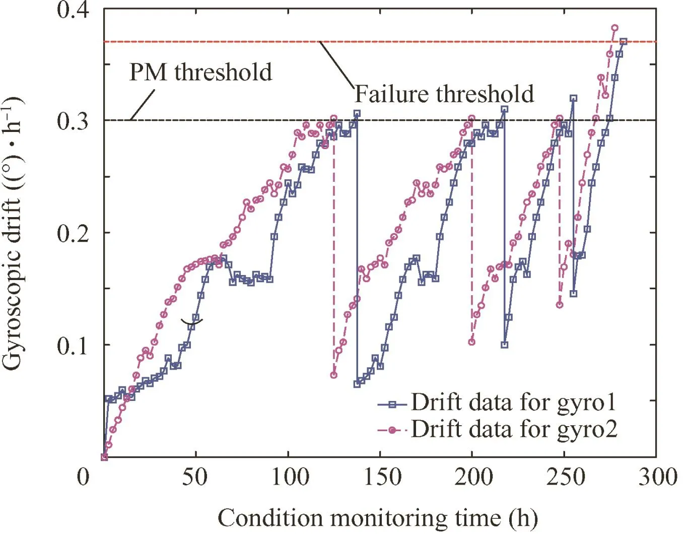
Fig.12 Degradation paths of gyros.

6.2.Results and comparison

Similarly,we can obtain the MLE values of the parameters（a，b，λ0，θ，σ2B）based on the simulation trajectory 1,as shown in Table 4.The estimation process of maintenance parameter is also similar to the last section,and hence,the maintenance parameter estimation is omitted here.

In order to verify the effectiveness of the RUL estimation method proposed in the paper,we select ti，j=150 h as the time for RUL estimation.According to the drift data for gyro 2,thefirst PM occurs at 125 h,and therefore,when ti，j=150 h,there exists one PM activity before ti，j.Based on the MC simulation algorithm proposed in the paper,Fig.13 provides the PDF of the RUL of the gyro 2 at ti，j=150 h for three methods.

From Fig.13,we can also find that the RUL of the gyro 2 is overestimated by method M2,and the RUL of gyro 2 is underestimated by the method M3.In other words,the estimated RUL by method M1is the best among these three methods,which illustrates the superiority of the method proposed in the paper.

We have considered the situation of 0≤i＜n above.In the following part,we will further consider the situation of i=n.Specifically,we select the time sequences as the RUL estimation points from 260 h to 280 h.We can obtain the PDFs of the RULs for gyro 2 by utilizing methods M1and M2.Fig.14 shows the estimated PDFs and means of the RULs of the gyro by methods M1and M2.

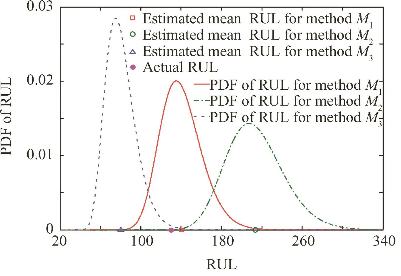
Fig.13 PDF of RUL at ti，j=150 h for three methods.

Table 4 Parameter estimation of gyros.

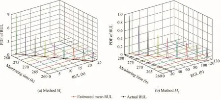
Fig.14 Estimated PDFs and means of RULs.

It can be readily seen from Fig.14 that the deviation between the estimated mean RUL by methodM2and the actual RUL seems so large that it cannot accurately estimate the RUL of the gyro.However,the deviation between the estimated mean RUL by methodM1and the actual RUL can be ignored after 265 h,and hence,the estimated mean RUL by methodM1can be used to re flect the actual RUL of the gyro,which further demonstrates the effectiveness and superiority of the RUL estimation method proposed in the paper.From the above discussion,we can conclude that it is necessary to consider the double influence of imperfect maintenance on the degradation level and the degradation rate for the RUL estimation of the gyro subjected to the intervention of imperfect maintenance activities.

7.Conclusions

For the equipment subjected to imperfect maintenance activities,this paper presented a degradation modeling and RUL estimation method considering the influence of imperfect maintenance activities on both degradation level and degradation rate.Specifically,a stochastic degradation model considering the influence of imperfect maintenance activities was established based on the diffusion process model.The parameters in the degradation model were estimated by MLE and Bayesian updating strategy based on the CM data and the maintenance data of the equipment.Further,the PDF of RUL was derived by the convolution operator under the concept of FHT.A numerical example and a practical case study were used to verify the effectiveness and superiority of the method proposed in the paper.From the experimental results,we can find that the method proposed in the paper can estimate the RUL accurately for the equipment subjected to the intervention of imperfect maintenance activities,which is beneficial to the optimal maintenance and spare parts ordering.Different from the existing work,our method considers the influence of the imperfect maintenance on both the degradation level and the degradation rate,which is more consistent with the actual situations.

This is a preliminary study and there are several further research topics which will be studied in the future.The first is to consider other distributions to characterize the degradation rate changing factor according to specific application background.The second is to make the maintenance or inventory decisions based on the prediction information obtained in this paper,since the main goal of the RUL estimation is to optimize the maintenance time and spare parts’ordering quantity by minimizing the operating cost or mitigating failure risk.

Acknowledgements

The work described in this paper was co-supported by the National Science Foundation ofChina (NSFC)(Nos.61573365,61603398,61374126,61473094,and 61773386),the Young Talent Fund of University Association for Science and Technology in Shaanxi,China,and the Young Elite Scientists Sponsorship Program(YESS)by China Association for Science and Technology(CAST).

1.Pecht MG.Prognostics and health management of electronics.New Jersey:John Wiley;2008.p.47–83.

2.Si XS,Wang W,Hu CH,Zhou DH.Remaining useful life estimation-a review on the statistical data driven approaches.Eur J Oper Res 2011;213(1):1–14.

3.Zio E,Compare M.Evaluating maintenance policies by quantitative modeling and analysis.Reliability Eng Syst Saf 2013;109(1):53–65.

4.Wang Y,Peng Y,Zi Y,Jin X,Tsui KL.A two-stage data-drivenbased prognostic approach for bearing degradation problem.IEEE Trans Ind Inf 2016;12(3):924–32.

5.Zio E,Peloni G.Particle filtering prognostic estimation of the remaining useful life of nonlinear components.Reliability Eng Syst Saf 2011;96(3):403–9.

6.Ye ZS,Chen N.The inverse Gaussian process as a degradation model.Technometrics 2014;56(3):302–11.

7.Wang XJ,Lin SR,Wang SP,Zhang C.Remaining useful life prediction based on the Wiener process for an aviation axial piston pump.Chin J Aeronaut 2016;29(3):779–88.

8.Tseng ST,Tang J,Ku LH.Determination of optimal burn-in parameters and residual life for highly reliable products.Naval Res Logistics 2003;50(1):1–14.

9.Ye ZS,Tsui KL,Wang Y,Pecht MG.Degradation data analysis using wiener processes with measurement errors.IEEE Trans Reliability 2013;62(4):772–80.

10.Si XS,Wang W,Hu CH,Zhou DH,Pecht MG.Remaining useful life estimation based on a nonlinear diffusion degradation process.IEEE Trans Reliability 2012;61(1):50–67.

11.Wang ZQ,Hu CH,Wang W,Si XS.An additive wiener processbased prognostic model for hybrid deteriorating systems.IEEE Trans Reliability 2014;63(1):208–22.

12.Huang ZY,Xu ZG,Wang WH,Sun YX.Remaining useful life prediction for a nonlinear heterogeneous Wiener process model with an adaptive drift.IEEE Trans Reliability 2015;64(2):687–700.

13.Wang D,Zhao Y,Yang F,Tsui KL.Nonlinear-drifted Brownian motion with multiple hidden states for remaining useful life prediction of rechargeable batteries.Mech Syst Signal Process 2017;93(7):531–44.

14.Wang ZQ,Wang W,Hu CH,Si XS,Zhang W.Aprognostic in formation-based order-replacement policy for a non-repairable criticalsystem in service.IEEE Trans Reliability 2015;64(2):721–35.

15.Pham H,Wang H.Imperfect maintenance.Eur J Oper Res 1996;94(1):425–38.

16.Labeau PE,Segovia MC.Effective age models for imperfect maintenance.Proc Inst Mech Eng Part O:J Risk Reliability 2010;225(1):117–30.

17.Castro IT,Mercier S.Performance measures for a deteriorating system subject to imperfect maintenance and delayed repairs.Proc Inst Mech Eng Part O:J Risk Reliability 2016;230(4):364–77.

18.Liu Y,Huang H.Optimal selective maintenance strategy for multi-state systems under imperfect maintenance.IEEE Trans Reliability 2010;59(2):356–67.

19.Nakagawa I,Yasui K.Optimal policies for a system with imperfect maintenance.IEEE Trans Reliability 1987;36(5):631–3.

20.Chang CK,Hsiang CL.An optimal maintenance policy based on generalized stochastic petri nets and periodic inspecting.Asian J Control 2010;12(3):364–76.

21.Van PD,Voisin A,Levrat E,Lung B.A proactive condition-based maintenance strategy with both perfect and imperfect maintenance actions.Reliability Eng Syst Saf 2015;133(11):22–32.

22.Wang ZQ,Hu CH,Wang W,Si XS.A simulation-based remaining useful life prediction method considering the influence of maintenance activities.Prognostics and system health management;2014 Aug 24–27,Hunan,China.p.284–9.

23.Zhang MM,Olivier G,Xie M.Degradation-based maintenance decision using stochastic filtering for systems under imperfect maintenance.Eur J Oper Res 2015;245(3):531–41.

24.Ponchet A,Fouladirad M,Grall A.Maintenance policy on a finite time span for a gradually deterioration system with imperfect improvement.Proc Inst Mech Eng Part O:J Risk Reliability 2011;225(2):105–16.

25.Moura MDC,Droguett EL,Firmino PRA,Ferreira RJ.A competing risk model for dependent and imperfect conditionbased preventive and corrective maintenances.Proc Inst Mech Eng Part O:J Risk Reliability 2014;228(6):590–605.

26.Zhou X,Xi L,Lee J.Reliability-centered predictive maintenance scheduling for continuously monitored system subject to degradation.Reliability Eng Syst Saf 2007;92(4):530–4.

27.You MY,Meng G.Residual life prediction of repairable systems subject to imperfect preventive maintenance using extended proportional hazards model.J Process Mech Eng 2012;226(1):50–63.

28.Guo CM,Wang W,Guo B,Si XS.A maintenance optimization model for mission-oriented systems based on Wiener degradation.Reliability Eng Syst Saf 2013;111(1):183–94.

29.Liao H,Elsayed EA,Chan LY.Maintenance of continuously monitored degrading systems.Eur J Oper Res 2006;175(2):821–35.

30.Gnedenko BV,Kolmogorov AN.Book reviews:limit distributions for sums of independent random variables.Biometrika 1963;50(272):281–90.

31.Xu C,Chang GS.Exact distribution of the convolution of negative binomial random variables.Commun Stat-Theory Methods 2016;46(6):2851–6.

32.Wang Y,Ye ZS,Tsui KL.Stochastic evaluation of magnetic head wears in hard disk drives.IEEE Trans Magn 2014;50(5):1–7.

33.Ye ZS,Chen N,Shen Y.A new class of Wiener process models for degradation analysis.Reliability Eng Syst Saf 2015;139:58–67.