GLOBAL EXISTENCE OF WEAK SOLUTIONS TO THE THREE-DIMENSIONAL FULL COMPRESSIBLE QUANTUM EQUATIONS∗

Boling Guo

(Institute of Applied Physics and Computational Math.,Beijing 100088,PR China)

Binqiang Xie

(The Graduate School of China Academy of Engineering Physics,Beijing 100088,PR China)

1 Introduction

In this paper,we are interested in the quantum fluid models.Such models can be used to describe super fluids[18],quantum semiconductors[7],weakly interacting Bose gases[11]and quantum trajectories of Bohmian mechanics[25].Since the numerical solution of the Schrodinger equation or the Wigner equation is very time consuming, fluid-type quantum models seem to provide a compromise between accurate and efficient numerical simulations.Moreover,quantum fluid models are formulated in macroscopic quantities like the current density,which can be measured.A hydrodynamic form of the single-state Schrodinger was already derived by Madelung[21].Later,the so-called quantum hydrodynamic equations were derived by Ferry and Zhou[7]from the Bloch equation for the density matrix.In[12]Gardner used the moment method to the Wigner equation leading to the full three-dimensional quantum hydrodynamic model(QHD).Jungel,Matthes and Milisic[15]obtained a new quantum hydrodynamic model using Levermore’s entropy minimization principle,which can be used to derive the full three-dimensional quantum hydrodynamic model including the vorticity matrix.Recently some dissipative quantum fluid models have been derived.In[13]the authors derived viscous quantum Euler models using a moment method in Wigner-Fokker-Planck equation.In[5],under some conditions,using a Chapman-Enskog expansion in Wigner equation,the quantum Navier-Stokes equations were obtained.

In the following,we consider a full quantum viscous quantum equations as follows:

with the total energy,the thermal diffusion flux and symmetric part of the velocity gradient respectively,

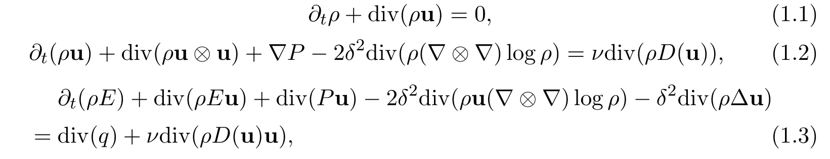
where ρ is the density of the fluid,u denotes the velocity field of the fluid,θ is the temperature of the fluid,P is the pressure field,q is the diffusion flux,κ is the thermal conductivity coefficient.The physical parameters are the Plank constant δ2＞ 0 and the viscosity constant ν ＞ 0.This system of equations corresponds to Garder’s QHD model[12]except for the dispersive terms δ2div(ρ∆u)and viscous terms νdiv(ρD(u)u).

Interestingly,quantum terms can be cancelled in the total energy equation.In fact,by substituting the above expression for the total energy density into equation(1.3)yields

System(1.1)-(1.3)is considered under initial conditions:

Here the functions ρ0and m0satisfy:

There have been a large amount of work on the global existence of weak solutions to the compressible Navier-Stokes equation without quantum effect,in the constant viscosity coefficients case.One of the main results of the nineties is due to Lions[19],who proved the global existence of weak solutions to the compressible Navier-Stokes system in the case of barotropic equations of state.Later,this result was extended to the somehow optimal case γ＞n/2 in[8]using oscillation defect measures on density sequences associated with suitable approximation solutions.For the full compressible Navier-Stokes equation,including the temperature equation,Feireisl[9]firstly proved the global existence of the so-called variational solutions to the full compressible Navier-Stokes and heat-conducting system.

Recently Bresch and Desjardins[2]made important progress in the case of viscosity coefficients depending on the density ρ,under some structure constraint on the viscosity coefficients,discovered a new entropy inequality(called BD entropy)which can yield global-in-time integrability properties on density gradients.This new structure was first discovered in[3]in the framework of capillary fluid.Later on,they founded that this BD entropy inequality also can be applied to the compressible Navier-Stokes equation without capillarity.By this new BD entropy inequality,they succeeded in obtaining global existence of weak solutions in the barotropic fluids with some additional drag terms.However,there are some difficulties without any additional drag term,as lack of estimates for the velocity.By introducing a new apriori estimate on smooth approximation solutions,Mellet and Vasseur[22]studied the stability of barotropic compressible Navier-Stokes equations.Unfortunately,they cannot construct smooth approximation solutions.Li and Xin[20]recently constructed some suitable approximate system which has smooth solutions satisfying the energy inequality,the BD entropy inequality,and the Mellet-Vasseur type estimate,therefore they completely solved an open problem.Independently,Vasseur and Yu[26]have proved the same result by constructing a different method.Bresch and Desjardins[4]also used this new entropy to obtain the global-in-time existence of weak solutions to the Navier-Stokes equations for viscous compressible and heat conducting fluids where the viscosity coefficients depend on the density.

On the other hand,there are few results about compressible Navier-Stokes equation with quantum effect.In[16],Jungel proved the global existence of weak solutions to the compressible quantum Navier-Stokes system in the case of barotropic equations of state when the scaled Plank constant is larger than the viscosity constant.In[6],Dong extended this result where the scaled Plank constant is equal to the viscosity constant,and in[17],Jiang showed that the result still holds when the viscosity constant is larger than the scaled Plank constant.In[14],Gisclon and Lacroix relaxed the assumption γ ＞ 3 to γ ＞ 1 by introducing a cold pressure.Very recently,Antonelli and Spirito[1]removed this additional cold pressure assumption in the sprit of the idea in[20].

In this paper we will study the global existence weak solutions to full quantum compressible Navier-Stokes equations(1.1)-(1.3)for the large initial data.In the treatment of systems(1.1)-(1.3),we need to overcome several mathematical difficulties.The first problem is lack of information of suitable estimates for the solutions.We use some relation about quantum terms in which these terms can be cancelled,thus we can obtain the basic energy estimate and the B-D entropy estimate which are key estimates to deduce the global-in-time existence of weak solutions to full compressible quantum Navier-Stokes equations.The second problem is the proof the compactness of the velocity sequences.In dealing with this obstacle,we introduce the stabilizing term in the form of cold pressure.This singular pressure prevents the appearance of vacuum.

1.1 Assumptions

This subsection deals with assumptions regarding physical coefficients,such as thermal conductivity and equation of state.

First of all,the thermal conductivity coefficient κ is assumed to satisfy:

where κ0=const.＞ 0,B ≥ 8.

Next,we assume that the above equations are of ideal polytropic gas type:

where R and Cµare two constant positive coefficients.Moreover,the additional pressure Pcand the internal energy ecare associated with the“zero Kelvin isothermal”.We require that ecis a C2nonnegative function on R+and the following constraint is satisfied

We also require that Pcis a continuous function satisfying the following growth condition

for positive constants c2,c3and γ−,γ+＞ 1.This cold pressure was firstly proposed in[4]to encompass plasticity and elasticity effect of solid materials,for which low densities may lead to negative pressures.By this modification,the compactness of velocity can be obtained.In later section we will use the notation:

1.2 Main result

Before we state the main result,we need to specify the definition of weak solutions given below.It is necessary to require that the weak solutions should satisfy the na-tural energy estimates and from the viewpoint of physics,the conservation laws on mass,momentum and energy also should be satisfied at least in the sense of distributions.Based on those considerations,the definition of reasonable global weak-in-time weak solutions is given as follows.

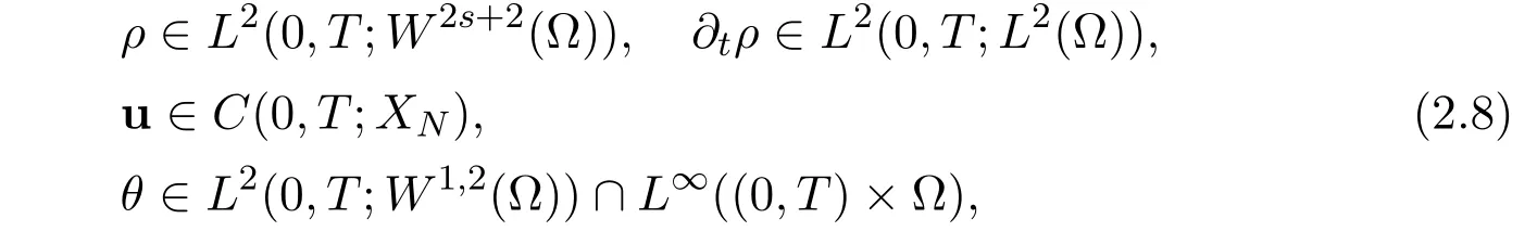
Definition 1.1A couple(ϱ,u,θ)is called a weak solution to system(1.1)-(1.3)if and only if for any positive number T,the following conditions are satisfied:

· ϱ,u,θ respectively belong to the classes

·the following identities are fulfilled:

–The continuity equation

is satisfied point wisely on[0,T]×Ω;

–the momentum equation

holds for any test smooth vector function ϕ such that ϕ(·,T)=0,where

–the total energy equation

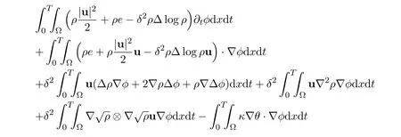
holds for any test smooth vector function ϕ such that ϕ(·,T)=0,where

Now our main result of this paper can be presented as follows:

Theorem 1.1Let Ω be the three-dimensional torus T3.Assume that κ,ec,Pcsatisfy the hypotheses(1.6)-(1.9).Let the initial datam0∈ L1(Ω),θ0∈ L4(Ω)such thatAssume the parameters γ ＞ 1 ,γ−＞3,B≥8.Let T＞0 be arbitrary.Then there exists a weak solution to(1.1)-(1.3)in Definition 1.1.Moreover,the density ρ ＞ 0 and the temperature θ＞ 0 a.e.in(0,T)×Ω.

2 Approximation

The aim of this section is to present two levels of approximation.First,we take ε,λ ＞ 0 and fix s to be a sufficiently large positive integer.Our aim is to consider the regularized problem given below,in which ε is the rate of dissipation in the continuity equation.We insert λ to the momentum equation to obtain the artificial smoothing operator λ∇∆2s+1ρ with s sufficiently large.Inspired by the works of Bresh and Desjardins,we introduce another regularization of the momentum λ∇∆2s+1(ρu).Note that by setting ε,λ → 0+,we recover our original problem.

We look for space periodic functions(ρ,ρu,θ)such that

to solve the following problem:

·The approximate continuity equation

is satisfied point wisely on[0,T]×Ω and the initial condition holds in the strong L2sense;here∈ C∞(Ω)is a regularized initial condition such that→ ρ0in Lγ+(Ω)for λ → 0+,and λ‖∇2s+1‖ → 0 for λ → 0+,with

·the weak formulation of the approximate momentum equation

holds for any test vector function ϕ ∈ L2(0,T;W2s+1(Ω))∩W1,2(0,T;W1,2(Ω))such that ϕ(·,T)=0;

·the weak formulation of the energy equality

and

are satisfied for any vector function ϕ ∈ C∞([0,T]× Ω)with ϕ(T,·)=0;here

We prove the following result.

Theorem 2.1Under the assumptions of Theorem 1.1 and the assumptions specified in this section,for any T ＞ 0,ε,λ ＞ 0,there exists a solution to problem(2.1)-(2.7)in the sence defined above.

Indeed,the proof of this result is far from being obvious.To prove Theorem 2.1 we have to introduce another level of approximation,based on regularization of certain quantities and finite dimensional projection(Faedo-Galerkin approximation)of the momentum equation.More precisely,we look for functions(ρ,u,θ)such that

to solve the following problem:

·The approximate continuity equation

is satisfied point wisely on[0,T]×Ω and the initial condition holds in the strong L2sense;hereis as above;

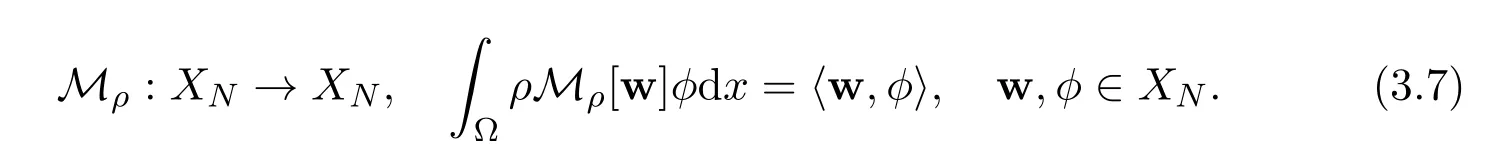
·the Faedo-Galerkin approximation for the weak formulation of the approximate momentum balance:Look for u∈C([0,T];XN)such that

holds for any test vector function ϕ ∈ XN,andwhereis an orthonormal basis in L2(Ω),such that ϕi∈ C∞(Ω)for all i∈ N;

·the approximate thermal energy equation:

is satisfied point wisely on[0,T]×Ω and the initial conditionia as above.

Theorem 2.2Let N∈N,ε,δ,λ＞0,and m0,,be as above.Under the assumptions of Theorem 1.1 and the assumptions specified in this section,for any T ＞ 0,ε,λ ＞ 0,there exists a solution to problem(2.9)-(2.11)in the sence defined above.

3 Basic Level of Appromation

This section is dedicated to the proof of Theorem 2.2.The strategy of the proof can be summarized as follows:

·Fix u(t,x)in the space C(0,T;XN)and use it to find a unique smooth solution ρ = ρ(u)to(2.9)and a unique strong solution θ= θ(ρ,u)to(2.11).

·Find the local-in-time solution to the momentum equation by a fixed point argument.

·Extend the local-in-time solution to the whole time interval using uniform estimates.

3.1 Continuity equation

We first prove the existence of a smooth,unique solution to the approximate continuity equation in the situation when the vector field u(x,t)is given and belongs to C([0,T];XN).

The following result can be proven by the Galerkin approximation and the well known statements about the regularity of the linear parabolic systems.

Lemma 3.1Let u ∈ C([0,T];XN)for N fixed andbe as above.Then there exists a unique classical solution to(2.9),that is ρ ∈ Vρ[0,T],where

Finally,for fixed N ∈ N,the function ρ is smooth in the space variable.

3.2 Temperature equation

The existence of unique solution to(2.11)can be proven as in[10],which is to transform and regularize equation(2.11)in such a way that the classical theory for quasilinear parabolic equations could be applied.We have the following lemma.

Lemma 3.2Let u ∈ C([0,T];XN)be a given vector field and ρ = ρube the unique solution of the approximate problem constructed in Lemma 3.1.Then there exists a unique strong solution to(2.11)which belongs to

3.3 Fixed point argument

At this stage,we are ready to show the existence of approximate solutions on a possibly short time interval(0,τ).We use the Schauder fixed point theorem to find a solution to the momentum equations.

More precisely,we prove that there exists a τ= τ(N)such that u solves the approximate momentum equation(2.10).To this purpose we consider the following mapping

which attain a solution to the following problem

where

and

Next,we consider a ball B in the space C([0,T];XN):

We need to show that the operator T is continuous and maps BRinto itself,provided τ is sufficiently small.First observe that

From estimates(3.8)and the estimates established in Lemmas 3.1 and 3.2,it follows that for sufficiently small τ,the operator T maps the ball BRinto itself.Moreover,T is a continuous mapping and its image of Lipschitz functions,thus it is compact in BR.It allows us to apply the theory of topological degree to infer that there exists at least one fixed point u solving(2.10)on[0,τ].

3.4 Uniform estimates and global in time solvability

In order to extend this solution to the whole time interval[0,T],we need a uniform bound of the solution.It follows from(3.5)that u is a continuously differentiable function,therefore,system(2.10)may be transformed to the following one

for any ϕ∈XN.Therefore we can test(3.9)by u.For the approximate momentum equation,using continuity equation,we obtain the kinetic energy balance

Adding this to equality(2.11),integrating it with respect to the space,then integrating the obtained result with respect to the time we obtain

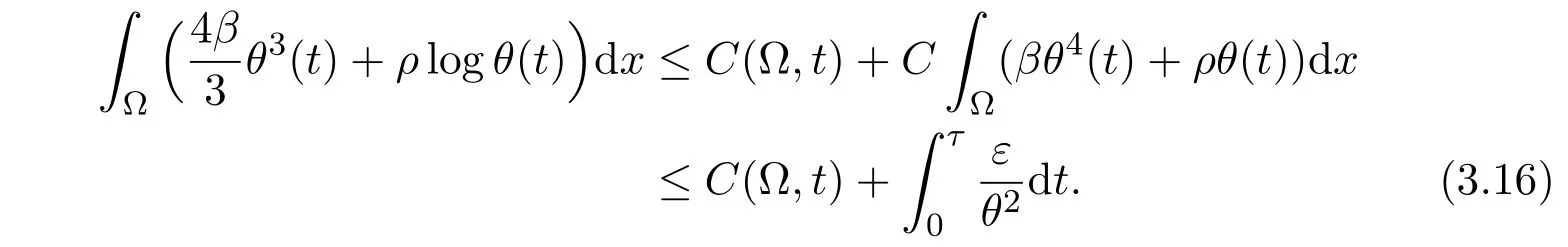
3.5 Entropy estimate

Our aim now is to derive a fundamental estimate for our system.It can be viewed as a total global entropy balance.

From Lemma 3.2 it follows in particular that θ is bounded from below by a constant.Therefore,dividing internal energy equation by θ is possible and the equation is

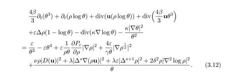
Integrating over Ω we get

Integrating the above inequality with respect to the time and adding it to equality(3.11),we get

To control the r.h.s,we take advantage of the fact of the heat conductivity coefficient.We write

To control the positive part of the entropy at time τ and its negative part at the initial time t=0 we note that

On the other hand,we easily verify that

which appears on the l.h.s.of(3.15).

Summarizing,we can show the following estimate

Taking s in the density-regularizing term to be sufficiently large,one can show that the density is separated from 0 uniformly with respect to all approximation parameter except for λ.This property was observed by Bresh and Desjardins in[11]where the case of single-component heat-conducting fluid was discussed.Recalling their analysis we may use the Sobolev embedding ‖ρ−1‖L∞(Ω)≤ C‖ρ−1‖W3,2(Ω)and

where the last term is bounded because of(3.18)and the assumption that γ−≥ 4.So,provided that 2s+1≥3 we have

3.6 Global-in-time existence of solutions

The uniform estimates for u can be summarized as follows

Moreover,the density ρ is bounded from below by a positive constant according to(3.20).By the equivalence of norms on the finite dimensional spaces XNwe can thus deduce the uniform bounds for u in C([0,τ);XN).Therefore we get a solution defined on[0,T]for arbitrary but finite T＞0.

4 Limit Passage in the Galerkin Approximation

The purpose of this section is to obtain the limit for N→∞in the equations of approximate system in Section 3.We start to summarize all the estimates that are uniform with respect to N derived mostly from(3.18)and its consequences.This will be done in Subsection 4.1,then in Subsection 4.2 we use these estimates to extract the weekly convergent subsequences and to prove that the limit N→∞can be performed.

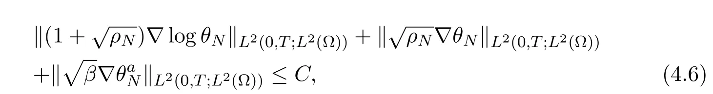
4.1 Estimates independent of N

Note that the above estimates are not only uniform with respect to the time but also with respect to N.From(3.16)and(3.18)we have

also from(3.11),we get that

In addition,we have the estimates following from the boundedness of the entropy production rate:

–the velocity estimates

–the density estimates

–the temperature estimates

Temperature estimates.One of the main consequences of(3.18)is(4.5)which,for κ satisfying(1.6),provides a priori estimates for the temperature

Kinetic energy estimates.We now integrate(3.10)with respect to the time and get

In the following we show the r.h.s of equality(4.8)are bounded.

and the r.h.s.is bounded provided 2s+1≥3.To see it,we write

and the boundness of the r.h.s follows from(3.20),(3.18)and the Cauchy inequality.

4.2 Passage to the limit with N

This subsection is devoted to the limit passage N→∞.Using estimates from the previous subsection we can extract weakly subsequences,whose limits satisfy the approximate system.It should be,however,emphasized that at this level we replace weak formulation of the thermal energy by the weak formulation of the total energy.

4.2.1 Strong convergence of the density and passage to the limit in the continuity equation

From(4.8)-(4.12)we deduce that

and

at least for a suitable subsequence.In addition the r.h.s.of the linear parabolic problem

is uniformly bounded in L2(0,T;W2s,2(Ω))and the initial condition is sufficiently smooth,thus,applying the Lp−Lqtheory to this problem we conclude thatis uniformly bounded in L2(0,T;W2s,2(Ω)).Hence,the standard compact embedding implies ρN→ ρ a.e.in(0,T)×Ω and therefore passage to the limit in the approximate continuity equation is straightforward.

4.2.2 Strong convergence of the temperature

For the temperature we have

note that at this level,the time-compactness can be proved directly from the internal energy equation(2.11).Indeed,due to the continuity equation,we have

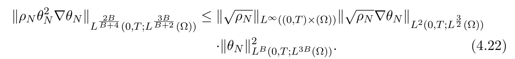
On the account of(4.5)and(4.8)the last 9 terms are bounded in L1((0,T)×Ω).Then it follows from(4.2),(4.7)and(4.9)that I1can be estimated as

and

where we used the interpolation

hence the last term is bounded provided B≥8.

For I2notice thattherefore using estimates(4.5)and(4.2)we verify that the most restrictive terms are bounded.Indeed,

with p＞1,further

Finally,since B ≥ 8,θB+1can be bounded using(4.20).

As a conclusion we have that

for some p,q ＞ 1.On the other hand,since∂tρ is uniformly bounded in L2(0,T;W2s,2(Ω)),ρ ＞ C(λ)and θ＞ 0,we have

thus an application of the Aubin-Lions lemma gives precompactness of the sequence approximating the temperature

for any 1≤ p′＜.

4.2.3 Passage to the limit in the momentum equation

Having the strong convergence of the density,we start to identify the limit for N→∞in the nonlinear terms of the momentum equation.

The convective term.First,one observes that

due to the uniform estimate(4.2)and the strong convergence of the density.Next,one can show that for anythe family of functions∫ρuϕdx isΩNNbounded and equi-continuous in C(0,T),thus via the Arzela-Ascoli theorem and density of smooth functions in L2(Ω)we get that

Finally,by the compact embedding L2(Ω)⊂ W−1,2(Ω)and the weak convergence of uNwe verify that

The capillarity term.We write it in the form

Due to(4.14)and the boundedness of the time derivative of ρN,we infer that

thus

for any ϕ ∈ C∞((0,T)× Ω).

The momentum term.We write it in the form

so the convergence established in(4.13)and(4.28)are sufficient to pass to the limit here.

Strong convergence of the density and temperature enables us to perform in the momentum equation(2.10)for any function ϕ∈C1([0,T];(XN))such that ϕ(T)=0 and by the density argument we can take all such test functions from C1([0,T];W2s+1(Ω)).

4.2.4 Passage to the limit in the internal energy balance equation

Passage to the limit in the terms νρ|D(u)|2, λ|∆s∇(ρu)|2, λε|∆s+1ρ|2and 2δ2ρ|∇2logρ|2requires a sort of strong convergence of these quantities.This will be deduced from the kinetic energy balance.For this purpose we need to show that u can be a test function in the limit momentum equation.Indeed,in(2.4)all terms are bounded due to estimate(4.8).Moreover,thanks to the lower bound of ρ we can verify that u is actually a continuous function with respect to the time and that it is continuously differentiable.To see this it is enough to differentiate(2.4)with respect to time and use the kinetic energy balance.

Now,using u as a test function and taking advantage of the fact that the limit continuity equation is satisfied point wisely,we obtain

for any t∈[0,T].On the other hand,duo to(3.10),we have

The comparison of these two expressions yields

and for all t∈[0,T]we have that

Having convergence of these norms and relevant weakly convergent sequences we deduce the strong convergence.Thus we are able to perform the limit passage in the internal energy equation(2.11)

for any smooth ϕ vanishing at t=T.

4.2.5 Passage to the limit in the total energy balance equation

Now we use uϕ as a test function in the limit momentum equation(2.4),using again the limit continuity equation and after integrating by parts we get

We apply the approximate continuity equation to the operator∆sand then test it by λdiv(∇∆sρϕ)in order to obtain

Now summing(4.33)with(4.34)and(4.35),and using the limit continuity equation to rewrite the termdivudxdt,we get the weak formulation of the total energy together with some terms which will appear in the subsequent limit passages

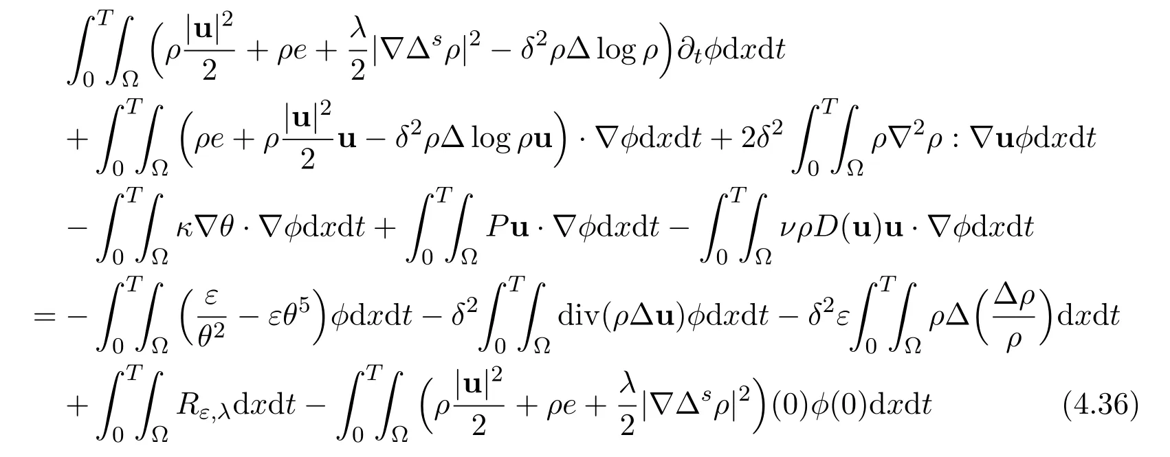
and

5 Derivation of the B-D Estimate

At this level we are left with only two parameters of approximation:ε and λ.From the so-far obtained a-priori estimates only the ones following from(3.11)and(3.18)were independent of these parameters.However having the ε-dependent estimate for∆s+1ρ allows us to derive a type of B-D estimate,from which it follow that this estimate depends only on λ.As a product,we will derive the energy estimate independent of λ.Note that so far in(4.8)we are only able to estimate the r.h.s.using the λ-dependent bounds for u.We will prove the following lemma.

Lemma 5.1For any positive constant r＞1,we have

in D′(0,T),

ProofThe proof is similar to that of[23].

In order to deduce the uniform estimates from(5.1)we need to control all the non-positive contribution to the l.h.s as well as the terms from the r.h.s.The ε−dependent terms can be bounded similarly to that in[23],so we fucus on the new aspect.

Estimate of∇P·∇ϕ.Using the assumption of P and∇ϕ=2∇logρ,we obtain

So the integral can be written

The first and second term is non-negative in view of the definition of πc,so it can be considered on the l.h.s.of(5.1)and we only need to estimate the third and the fourth terms as follows:

and the first term in(5.5)is bounded for B≥8 while the second(5.5)one can be estimated differently in two cases:

(i) ρ ≥ 1,then ρ−1≤ 1 and ρ−2|∇ρ|2≤ ρ−1|∇ρ|2which is then bounded by applying to the Gronwall inequality to(5.1);

(ii) ρ ＜ 1,then ρ−γ≥ 1 andwhich is absorbed by the analogous term from the l.h.s.of(5.1).

Estimate of(Pm+)divu.By the assumption of Pm,we have

Furthermore,by the Young’inequality

the last term in the right hand side of the above inequality can be written

On the account of(4.6),θ ∈ L2(0,T;L6(Ω)).Moreover,the Sobolev imbedding theorem implies that the right hand side of(5.6)is bounded whereas the first term can be absorbed by the left hand side.

The radiative term is slightly more difficult,however,we still can writefor 1 ≤ p ≤ 6,hence the last term in

and the last two terms are estimated by the r.h.s.of(5.1)and(5.3),while the boundedness of the first one follows from(4.1)and(4.8).

Estimate ofλ∆s∇(ρu):∆s∇2ρ.We have

therefore for r sufficiently large with rλ−1＞ c,both terms in the right hand side of(5.9)are bounded by the r.h.s.of(5.1).

6 Estimates Independent of ε,λ,Passage to the Limit ε,λ → 0

In this section we first present the new uniform bounds arising from the estimate of B-D entropy,performed in Section 5,and then let the last two approximation parameters be 0.Note that the limit passage λ → 0,ε→ 0 could be done in a single step,however,for transparency of this proof we do it separately.

We complete the set uniform bounds by

moreover

The uniform estimates for the velocity vector field are

and the constants from the r.h.s are independent of ε and λ.

We now present several additional estimates of ρ and u based on imbedding of Sobolev spaces and simple interpolation inequalities.Notice that the B-D estimates can be proven exactly as in the paper of Bresch and Desjardins devoted to the Navier-Stokes-Fourier system.However,for completeness,we recall them below.

Further estimates ofρ.From(5.1)we deduce that there exist functions ξ1(ρ)= ρ for ρ ＜ (1 − δ),ξ1(ρ)=0 for ρ ＜ 1 and ξ2(ρ)=0 for ρ ＜ 1,ξ2(ρ)= ρ for ρ ＞ (1+δ),δ＞ 0,such that

additionally in accordance with(5.3),where we are allowed to use the Sobolev imbeddings,thus

From(5.1)we can also derive the following estimates:

and

Similarly,we obtain

Remark 1Note in particular that the first of estimate(6.4)implies that

Estimate of the velocity vector field.We use the Holder inequality to write

Next,by a similar argument

Since γ−＞ 3 ,we see in particular that u ∈ L52(0,T;L52(Ω))uniformly with respect to ε and λ.

Remark 2By the estimates of the temperature we can deduce that

6.1 Passage to the limit with ε→ 0

With the B-D estimate at hand,especially with the bound on ∆s+1ρεin L2((0,T)×Ω),which is now uniform with respect to ε,we may perform the limit passage similarly to that in previous step.Indeed,the uniform estimates allow us to extract subsequences,such that

therefore

The strong convergence of the density as well as the velocity(since ρε)can be obtained identically as in previous step.Therefore we focus only on the strong convergence of the temperature and the limit passage in the total energy balance.

From(3.18)and(4.7),it follows that

and

The pointwise convergence of the temperture is deduced from the version of the Aubin-Lions lemma,see[23].

Lemma 6.1Let vεbe a sequence of functions bounded in L2(0,T;Lq(Ω))and in L∞(0,T;L1(Ω)),where q＞.Furthermore,assume that

where gεis bounded in L1(0,T;W−m,r(Ω))for some m ≥ 0,r ＞ 1 independent of ε.Then there exists a subsequence vεwhich converges to v strongly in L2(0,T;W−1,2(Ω)).

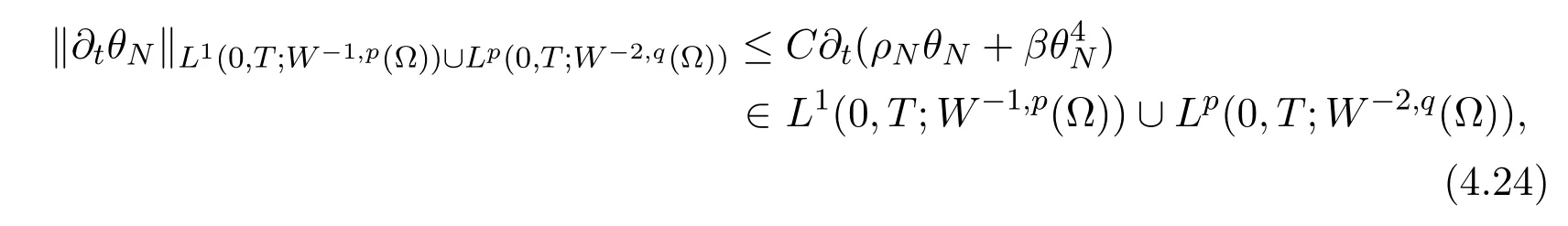
We will apply this lemma to vε=ρεθε+.Then,we can repeat the estimates from(4.17)to(4.24)to check that

Moreover,the r.h.s.is bounded in L1(0,T;W−1,p(Ω))∪L1(0,T;W−2,q(Ω))for some p,q ＞ 1.Therefore,the above lemma and the strong convergence of ρεimply in particular that

On the other hand,we also know that θε→ θ weakly in L2(0,T;W1,2(Ω)),therefore a simple argument based on the monotonicity of f(x)=x4implies strong convergence of θεin Lq(0,T;L3q(Ω))for any q ＜ B.

Let us finish this subsection with the list of the limit equations:

–the continuity equation

is satisfied pointwisely on[0,T]×Ω;

–the momentum equation

holds for any test function ϕ ∈ L2(0,T;W2s+1(Ω))∩ W1,2(0,T;W1,2(Ω))such that ϕ(·,T)=0;

–the total energy equation

holds for any test function ϕ ∈ L2(0,T;W2s+1(Ω))∩ W1,2(0,T;W1,2(Ω))such that ϕ(·,T)=0 and

Moreover,using the lower semicontinuity of norm and passing to the limit in(4.33),

is satisfied in the sense of distributions on(0,T)×Ω.

6.2 Passage with λ → 0

In this section,from the uniform estimate derived in the previous section and Lion-Aubin lemma,we deduce the strong compactness of the sequenceandshowed below.

Lemma 6.2Under the hypothesis of Theorem 1.1,we have for a fixed δ

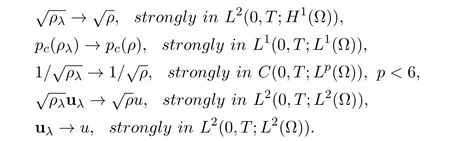
ProofFirstly we show the strong convergence of the sequenceThe estimate≤c together with the conservation of the mass‖ρλ(t)‖L1(Ω)= ‖ρλ(0)‖L1(Ω)gives the L∞(0,T;H1(Ω))bound,we also have the L2(0,T;H2(Ω))bounded.Next,noticing that

we can show that

Thus we can apply the Lion-Aubin lemma to obtain the strong convergence oftoin L2(0,T;H1(Ω)).

Sobolev imbedding implies that ρλis bounded in L∞(0,T;L3(Ω))and therefore

The continuity equation thus yields ∂tρλbounded in L∞(0,T;W−1,3/2(Ω)).Moreover,sinceis bounded in L∞(0,T;L3/2(Ω)),hence the compactness of ρλin C([0,T];(Ω)).

Next we show the strong convergence of the sequence of the cold pressure.From the previous section we can yield pc(ρλ)is bounded in L5/3((0,T)× Ω).Since we already know that pc(ρλ)converges almost everywhere to pc(ρλ),those bounds yield the strong convergence of pc(ρλ)in((0,T)×Ω).

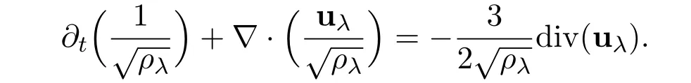
Moreover,we deduce the strong convergence of the sequence of,and rewrite the equation as follows

Using the pervious estimates,we have

Moreover,we derive the strong convergence of the sequences of ρλuλandand notice that

Using the momentum equation,we can get information on ∂t(ρλuλ)and therefore through the the Lion-Aubin lemma to obtain the almost everywhere convergence of ρu.From this and the almost everywhere convergence ofwe get the sequenceconverges almost everywhere tothen using the uniform boundedness of the sequencebelonging to Lp′([0,T];Lq′(Ω))for p′,q′＞ 2,we obtain the strong convergence of the sequence

Combing the strong convergence oftoin C([0,T];Lp(Ω))for p ＜ 6 with the strong convergence of the sequencein L2(0,T;L2(Ω)),we deduce that uλconverges to u in L2(0,T;Lp(Ω))for all p＜ 3/2.Recalling the uniformwe deduce that uλconverges strongly to u in L2(0,T;L2(Ω)).The proof is completed.

When we have these estimates,we can pass to the limit in

Strong convergence of the temperature.The difference with the previous chapter is that we cannot use the higher order either for the velocity or for the density in order to deduce the boundedness of the time derivative of temperature in a appropriate space.However,the idea of proving compactness of the temperature is,as previously,to apply Lemma 6.2 withTherefore,our next aim is to check that its assumptions are satisfied uniformly with respect to λ.

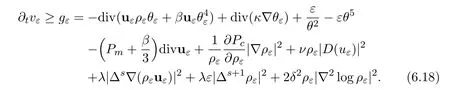
First,note that vλis bounded in L2(0,T;Lq(Ω))and in L∞(0,T;L1(Ω)),where q＞,uniformly with respect to λ.Indeed,it follows directly from(4.2)and(4.6).Further,one deduces that ∂tvλ≥ gλ,where gλhas the following form

and is bounded in L1(0,T;W−m,r(Ω))for some m ≥ 0,r ＞ 1 independent of λ.Indeed,this can be estimated,similarly to(4.18)-(4.22)except for the terms that contains velocity.For them we may write

on account of(4.20)and(6.10),further

For the internal pressure we have

Passage to the limit in the nonlinear terms.The last step in the limit passage λ → 0 is the verification of convergence in the nonlinear terms of the system.The most demanding of them are in the energy equation,and we only justify the limit passage in this case.The correction of energy λ∇2s+1ρλ→ 0 strongly in L2((0,T)×Ω),therefore the energy

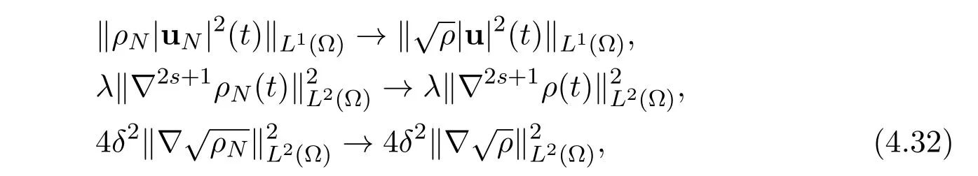
converges to E due to the strong convergence of ρλ,θλ,and the weak convergence of∆ρλ.Similarly uλρλθλ,and Puλconverge weakly to uρθ,ρu3and Pu respectively,due to uniform bounds in Lp((0,T)×Ω)for p＞ 1 from Lemma 6.2,the strong convergence of ρλ,θλand uλ.

For the quantum flux,we pass to the limit in ρλ∆uλnamely in terms with uλ∆ρλ,uλ∇ρλor uρλ,Since uλconverges strongly to u in L2(0,T;L2(Ω)), ρλand ∇ρλconverges strongly to ρ and ∇ρ in L2(0,T;L2(Ω))respectively and ∆ρλconverges weakly to ∆ρ in L2(0,T;L2(Ω)).As a consequence,ρλ∆uλconverges weakly to ρ∆u.

The stress quantum flux ρλuλ∇2logρλconverges weakly to ρu∇2ρ.Indeed,

since uλconverges strongly to u in L2(0,T;L2(Ω)),ρλand ∇ρλconverges strongly to ρ and ∇ρ in L2(0,T;L2(Ω))respectively and ∆ρλconverges weakly to ∆ρ in L2(0,T;L2(Ω)),thus we complete this limit process.

Limit passage in the heat flux term κ∇θλcan be performed directly,since it involves only the sequences ρλand θλwhich are strongly convergent,and a sequence∇θλwhich converges to∇θ in L2((0,T)×Ω).

We are now ready to prove that the corrector term Rλconverges to 0 strongly in L1((0,T)×Ω)as λ → 0.In fact,we have

thus we must show that the right hand side of the above inequality converges to 0.But this is evident,since one can use the Gagliardo-Nirenberg interpolation inequality and uniform bounds for ρλuλin L∞(0,T;L3/2(Ω);for ρλin L∞(0,T;L3(Ω);and forin L2(0,T;W2s+1,2(Ω)and L2(0,T;W2s+2,2(Ω),respectively.This finishes the proof of the main Theorem 1.1.

[1]P.Antonelli,S.Spirito,Global existence of finite energy weak solutions of quantum Navier-Stokes equations,Archive for Rational Mechanics Analysis,225:3(2017),1161-1199.

[2]D.Bresch,B.Desjardins,Some diffusive capillary models for Korteweg type,Comptes Rendus Mecanique,11:11(2004),881-886.

[3]D.Bresch,B.Desjardins,C.K.Lin,On some compressible fluid models: Korteweg,lubrication,and shallow water systems,Comm.Partial Differential Equations,28(2003),843-868.

[4]D.Bresch,B.Desjardins,On the existence of global weak solutions to the Navier-Stokes equations for viscous compressible and heat conducting fluids,J.Math.Pures Appl.,87(2007),57-90.

[5]S.Brull,F.Mehats,Derivation of viscous correction terms for the isothermal quantum Euler model,Z.Angew.Math.Mech.,90:3(2010),219-230.

[6]J.Dong,A note on barotropic compressible quantum Navier-Stokes equations,Nonlinear Analysis:Real World Applications,73(2010),854-856.

[7]D.Ferry,J.R.Zhou,Form of the quantum potential for use in hydrodynamic equations for semiconductordevice modeling,Phys.Rev.B,48(2015),7944-7950.

[8]E.Feireisl,A.Novotny,H.Petzeltova,On the existence of globally defined weak solutions to the Navier-Stokes equations,Journal of Mathematical Fluid Mechanics,3(2001),358-392.

[9]E.Feireisl,On the motion of a viscous,compressible,and heat conducting fluid,Indiana Uiv.Math.J.,53(2004),1707-1740.

[10]E.Feireisl,A.Novotny,Singular Limits in Thermodynamcs of Viscous Fluids,Advances in Mathematical Fluid Mechanics,2009.

[11]J.Grant,Pressure and stress tensor expressions in the fluid mechanical formulation of the Bose condensate equations,J.Phys.A:Math.,Nucl.Gen.,6(1973),L151-L153.

[12]C.Gardner,The quantum hydrodynamic model for semiconductor devices,SIAM J.Appl.Math.,54(1994),409-427.

[13]M.Gualdani,A.Jungel,Analysis of the viscous quantum hydrodynamic equations for semiconductors,European J.Appl.Math.,15(2005),577-595.

[14]M.Gisclon,I.Lacroix,About the Barotropic compressible quantum Navier-Stokes equations,http://arxiv.org/abs/1412.1332v1.

[15]A.Jungel,D.Matthes,J.P.Milisic,Derivation of new quantum hydrodynamic equations using entropy minimization,SIAM J.Appl.Math.,67(2006),46-68.

[16]A.Jungel,Global weak solutions to compressible Navier-Stokes equations for quantum fluids,SIAM J.Math.Anal.,42(2010),1025-1045.

[17]F.Jiang,A remark on weak solutions to the barotropic compressible quantum Navier-Stokes equations,Nonlinear Analysis:Real World Applications,12(2011),1733-1735.

[18]M.Loffredo,L.Morato,On the creation of quantum vortex lines in rotating He II,IL Nouvo Cimento B,108(1993),205-215.

[19]P.L.Lions,Mathematical Topics in Fluid Mechanics,vol.II,Compressible Models,Clarendon Press,Oxford,1998.

[20]J.Li,Z.P.Xin,Global existence of weak solutions to the barotropic compressible Navier-Stokes flows with degenerate viscosities,http://arxiv.org/abs/1504.06826v1.

[21]E.Madelung,Quantentheorie in hydrodynamischer form,Z.Physik,40(1927),322-326.

[22]A.Mellet,A.Vasseur,On the isentropic compressible Navier-Stokes equations,Comm.Partial Differential Equations,32(2005),431-452.

[23]P.B.Mucha,M.Pokoorny,E.Zatorska,Heat-conducting,compressible mixtures with multicomponent diffusion:construction of a weak solution,arXiv:1401.5112v2.

[24]P.B.Mucha,M.Pokoorny,E.Zatorska,Approximation solutions to model of twocomponent reactive flow,Discrete Contin.Syst.Ser.S,7(2014),1079-1099.

[25]R.Wyatt,Quantum Dynamics with Trajectories,Springer,New York,2005.

[26]A.Vasseur and Ch.Yu,Existence of global weak solutions for 3D degenerate compressible Navier-Stokes equations.Invent.Math.,206:3(2016),935-974.