FLIC:Fast linear iterative clustering with active search

Jiaxing Zhao,Ren Bo(),Qibin Hou,Ming-Ming Cheng,and Paul Rosin

Abstract In this paper,we reconsider the clustering problem for image over-segmentation from a new perspective.We propose a novel search algorithm called“activesearch” which explicitly considersneighbor continuity.Based on this search method,we design a back-and-forth traversal strategy and a joint assignment and update step to speed up the algorithm.Compared to earlier methods,such as simple linear iterative clustering(SLIC)and its variants,which use fixed search regions and perform the assignment and the update steps separately,our novel scheme reduces the number of iterations required for convergence,and alsoprovidesbetterboundariesin theoversegmentation results.Extensive evaluation using the Berkeley segmentation benchmark verifies that our method outperforms competing methods under various evaluation metrics.In particular,our method is fastest,achieving approximately 30 fps for a 481×321 image on a single CPU core.To facilitate further research,our code is made publicly available.

Keywordsimage over-segmentation;SLIC;neighbor continuity;back-and-forth traversal

1 Introduction

Superpixels,generated by image over-segmentation,can take the place of pixels as the fundamental units in various computer vision tasks,including image segmentation[1],image classification[2],3D reconstruction[3],object tracking[4],etc.Such a technique can greatly reduce computational costs,avoid under-segmentation,and reduce the in fluence of noise.Clearly,efficiently generating superpixels plays an important role in many vision and image processing applications.

Many classical methods have been developed for superpixel generation,including FH[5],Mean Shift[6],and Watershed[7]methods.The lack of compactness and the irregularity of the resulting superpixels restrict their application,especially when contrast is poor or shadows are present.To solve the above-mentioned problems,Shi and Malik proposed the normalized cuts(NC)method[8]which generates compact superpixels.However,this method does not follow image boundaries very well,and the computational cost is high. The GraphCut method[9,10]regards the segmentation problem as an energy optimization process.It solves the compactness problem by using min-cut/max- flow algorithms[11,12],but their parameters are hard to control.The Turbopixel method[13]provides another approach to solving the compactness problem.However,the inefficiency of the underlying levelset method[14]restricts its application.Van den Bergh et al.[15]proposed an energy-driven algorithm,SEEDS,whose results follow image boundaries well,but unfortunately it suffers from irregularity and the number of superpixels output is hard to determine.The ERS method[16]performs well on the Berkeley segmentation benchmark,but has a high computational cost that limits its practical use.

Achanta et al.[17]proposed a linear clustering based algorithm called SLIC;it generates superpixels based on Lloyd's algorithm[18](also known as Voronoi iteration or thek-means method). For speed,in the assignment step of SLIC,each pixel pis associated with those cluster seeds whose search regions overlap its location.This strategy is also adopted by most subsequent works based on SLIC.SLIC is widely used in various applications[4]because of its high efficiency and good performance.Inspired by SLIC,Wang et al.[19]implemented an algorithm called SSS that considers the structural information within images.It uses geodesic distance[20]computed by geometric flows instead of the simple Euclidean distance.However,its efficiency is poor because of the high computational cost of measuring geodesic distances.Very recently,Liu et al. [21]proposed the Manifold SLIC method that generates content-sensitive superpixels by computing a centroidal Voronoi tessellation(CVT)[22]in a special feature space.This advanced technique is much faster than SSS but still slower than SLIC due to the cost of its mapping,splitting,and merging processes.In summary,the above-mentioned methods improve the results by either using more complicated distance measurements or by providing more suitable transformations of the feature space.However,the assignment and update steps within these methods are performed separately,leading to a low convergence rate.

2 Proposed approach

In this paper,we consider the over-segmentation problem from a new perspective. Each pixel in our algorithm is allowed to actively search for the superpixel to which it belongs,according to its neighboring pixels—see Fig.1.During this process,the seeds of the superpixels can be adaptively changed,which allows our assignment and update steps to be performed jointly.This property enables our approach to converge rapidly.To sum up,the main advantages of our new approach are:

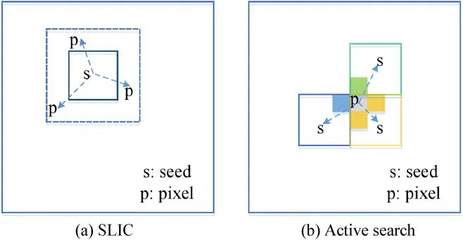
Fig.1 (a)Search method used in SLIC.Each seed only searches over a limited region to reduce computational cost.(b)Our active search method.Each pixel decides its own label by searching its surroundings.

· Good awareness of neighboring-pixel continuity,leading to results with good boundary sensitivity regardless of image complexity and contrast.

· Joint performance of the assignment and update steps,providing rapid convergence(in just two iterations).Our method has the highest speed of any superpixel segmentation approach,with better performance according to a variety of metrics evaluated on the Berkeley segmentation benchmark.

3 Preliminaries

Before introducing our approach that allows adaptive search regions and joint assignment and update steps,we first brie fly recap the standard SLIC algorithm with fixed search regions and separate steps.This approach improves upon Lloyd's algorithm,reducing the time complexity fromO(KN)toO(N),whereK is the number of superpixels andNis the number of pixels.

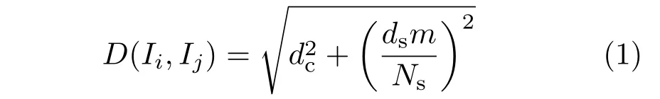
wheremis a variable that controls the weight of the spatial term,andNs=T.Variablesdsanddcare respectively the spatial and color distances,given by

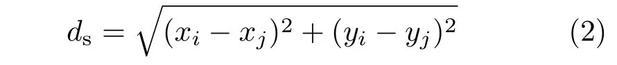
and

In the update step,SLIC recomputes the center of each superpixel and moves the seeds to these new centers.Overall,it obtains the over-segmentation results by iteratively performing the assignment and update steps.

Variants ofSLIC use a similar approach.They improve upon the performance of SLIC by using better distance measures or more suitable transformation functions between color space and spatial space.However,in these algorithms,each search region is fixed during the assignment step within each loop,and the relationships between neighboring pixels are largely ignored when allocating pixels to superpixels. Separately performing the assignment step and the update step causes delayed incorporation of pixel label changes.

Since superpixel computation is typically used as the first step of other vision applications,the rapid generation of superpixels with good boundaries is a crucial problem.Here,unlike previous algorithms[17,21],we consider this problem from a new point of view,in which only surrounding pixels are considered for determining the label of the current pixel.Each pixel actively selects which superpixel it should belong to in a back-and-forth order to provide better determination of over-segmentation regions.Moreover,the assignment step and the update step are performed jointly.Very few iterations are required for our approach to converge.An overview of our algorithm is provided in Algorithm 1.

3.1 Problem setup

Given the desired number of superpixelsKand an input imageI=,whereNis the number of pixels,our goal is to produce a series of disjoint small regions(or superpixels). Following most previous works[17],the original RGB color space is transformed to the more useful CIELAB color space.Thus,each pixelIiin an imageIcan be represented in a five dimensional space:

We first divide the original image into a regular grid containingKelementswith step lengthυ=as in Ref.[17],and the initial label for each pixel Iiis assigned as

We initialize the seedSkinGkat its centroid.Therefore,Skcan also be defined as being in the same five dimensional space:

?

3.2 Label decision

In most natural images adjacent pixels tend to share the same labels,i.e.,neighboring pixels have natural continuity.Thus,we propose an active search method to leverage as much of this a priori information as possible.In our method,unlike most previous approaches[17,21],the label of each pixel is only determined by its neighbors.We compute the distances between the current pixel and the seeds of its four or eight adjacent pixels—see Fig.1.Specifically,for a pixelIi,our assignment principle is

whereAiconsists ofIiand its four neighboring pixels,andSLjisIj's corresponding superpixel seed.We use Eq.(1)to measure the distance D(Ii,SLj).

Since each pixel can only be assigned to a superpixel containing at least one of its neighbors,local pixel continuity has a stronger effect in our proposed strategy,allowing each pixel to actively assign itself to one of its surrounding closely connected superpixel regions.The advantages of such a strategy are clear:firstly,the nearby assignment principle can avoid the occurrence of too many isolated regions,indirectly preserving the desired number of superpixels.Secondly,this assignment operation is not limited by a fixed range in space,resulting in better superpixel boundary compliance even when very complicated content leads to irregular superpixel shapes.Furthermore,during the assignment process,the superpixel centers are also self-adaptively modified,leading to faster convergence.Detailed demonstration and analysis are given in Section 4.5.It is worth mentioning that the neighbors of the internal pixels in a superpixel normally share the same labels,so it is unnecessary to process them further,allowing us to process each superpixel extremely quickly.

3.3 Traversal order

The traversal order plays a very important role in our approach:an appropriate scanning order may lead to a visually better segmentation.As explained in Section 3.2,the label of each pixel only depends on the seeds of its surrounding pixels.Thus,in a superpixel,the label of the current pixel is directly or indirectly related to those pixels that have already been processed.To better take advantage of this avalanche effect,we adopt a back-and-forth traversal order as in PatchMatch[23],in which the pixels that are processed later will benefit from updates to previously processed pixels.Figure 2 illustrates this process.In the forward pass,the label decision for each pixel considers the information from the top surrounding pixels of the superpixel,and similarly,the backward pass will provide the information from the bottom surrounding pixels of the superpixel.With such a scanning order,all the surrounding information can be taken into consideration,yielding better segments.

While an arbitrary superpixel may have an irregular shape instead of a simple rectangle or square,we use a simple strategy to traverse the whole superpixel.We first find a minimum bounding box within which all its pixels are enclosed,as shown in Fig.2.We then perform the scanning process for all pixels in the corresponding minimum bounding box and only deal with those pixels that are within the superpixel.

3.4 Joint assignment and update step

It is common in existing methods,such as SLIC[17],that the assignment and update steps are performed separately,leading to delayed feedback from pixel label changes to superpixel seeds.An obvious problem of such a strategy is that many(normally more than if ve)iterations are required before convergence.In our approach,based on the assignment principle in Eq.(7),we use a joint assignment and update strategy which performs these two steps at a finer granularity.This approach is able to adjust the superpixel seed center position on the fly,significantly reducing the number of iterations needed for convergence.Since most clustering-based superpixel methods use the centroidal Voronoi tessellation(CVT),we first briefly introduce the CVT and then describe our method.

whered(Ii,Sk)is an arbitrary distance measure from pixelIito the seedSk.The Voronoi diagramVD(S)is defined by

A CVT is then defined as a Voronoi diagram whose generator point of each Voronoi cell is also its center of mass.The CVT is usually obtained by heuristic algorithms,such as Lloyd's algorithm,iteratively performing updates after each assignment step until convergence is reached.

In our approach,on account of our novel label decision strategy as shown in Eq.(7),we are able to jointly perform the update step and the assignment step instead of separately.More specifically,after pixelIiis processed,if its label is changed to,say,Lj,we immediately update the current seedSLiusing the following equation:

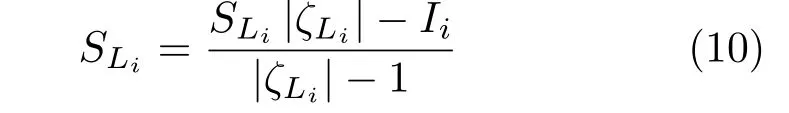
where|ζLi|is the number of pixels in superpixelζLi,and update SLjusing the following equation:

The bounding box ofζLjis also updated accordingly.

Fig.2 Scanning order for each superpixel.Gray regions enclosed by blue lines represent superpixels.Red dashed rectangles denote their corresponding bounding boxes.We first scan the bounding box from left to right and top to bottom(b)and then in the opposite direction(c).The shape of each superpixel may change,whereupon we update the bounding box(d)if necessary.

As the above updates only contain very simple arithmetic operations,they can be performed very quickly.Such an immediate update will help later pixels make a better choice during assignment,leading to better convergence.Figure 10 given later illustrates the speed of convergence of our approach.

3.5 Superpixel processing order

In our method,superpixels are processed independently.Thus,the superpixel processing order will affect the performance of the method;label changes affect the surrounding pixels.However,we do not want current pixel changes to affect the superpixels we have already processed.Therefore,we give priority to those complex superpixels in which many pixels labels will be changed,processing them first and then simple superpixels later.Superpixels which have a uniform color are simple,and almost no pixels labels need to change.

We use color entropy to define the complexity of superpixels.We calculate it using the following formulation(15):

where|ζLi|is the number of pixels in superpixelζLi,pis a three-dimensional vector in lab color space,and p is the mean of p in superpixel ζLi.

After determining the entropy of all superpixels,we process them in descending order of entropy.We later demonstrate the benefits of this processing order.

4 Experiments

Our method has been implemented in C++on a PC with a 4.0 GHz Intel Core i7-4790K CPU with 32 GB RAM,and 64 bit operating system.We compare our method to various previous and state-of-theart works,including FH[5],SLIC[17],Manifold SLIC[21],SEEDS[15],and ERS[16],using the BSDS500 benchmark and the evaluation methods proposed in Refs.[24,25].As the source codes used in evaluation of the above works may not be the same as the reported versions,we may observe performance differences from the original during evaluation.For fair comparison,we uniformly use publicly available source code[24,25]for all methods.As in previous research in the literature[19,21],we mainly evaluate all algorithms on 200 randomly selected images of resolution 481×321 from the Berkeley dataset[24].In addition,we compared our method with other stateof-the-art methods on the Pascal Context dataset[26].

4.1 Datasets

The Berkeley dataset is the most common dataset in the area of image segmentation and boundary detection. The Pascal Context dataset includes a set of additional annotations to the PASCAL VOC 2010 dataset[27].It goes beyond the original PASCAL semantic segmentation task by providing annotations for the whole scene and is mainly intended for semantic segmentation and object detection.Hence,we only perform an ablation study on the Berkeley dataset and compare our method with other methods on both datasets.We randomly selected six images and corresponding ground-truths from the BSDS(Fig.3)and Pascal Context datasets(Fig.4).

As we can see,the images in the Pascal Context are more realistic,while the annotations for the BSDS dataset are more detailed.

4.2 Parameters

Our approach requires three parameters to be set.The first is the number of superpixelsK.One of the common advantages of clustering-based algorithms is that the desired number of superpixels can be directly chosen by setting the clustering parameterK.The second parameter is the spatial distance weightm.It has a large effect on the smoothness and compactness of superpixels.We show that performance increases asmdecreases.However,makingmtoo small can also lead to irregularity of superpixels.To achieve a good trade-offbetween compactness and speed,in the following experiments,we setm=5 as default.The last parameter is the maximum number of iterations itr.Here we setitr=2 by default to balance time taken and result quality.We emphasise that,to make a fair comparison,we optimize the parameters for each method to maximize its recall value for the BSDS500 benchmark.

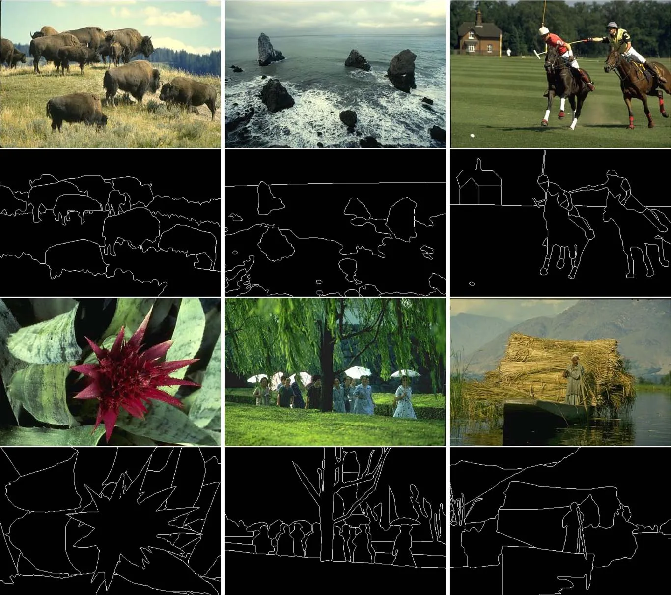
Fig.3 Images and ground-truths for the BSDS dataset.Rows 1,3:original images.Rows 2,4:corresponding annotated edges.

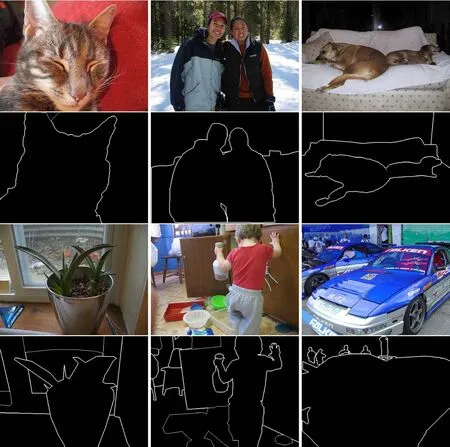
Fig.4 Images and ground-truths for the Pascal Context dataset.Rows 1,3:original images.Rows 2,4:corresponding annotated edges.

4.3 Comparison using BSDS dataset

Our approach outperforms previous methods that have similar computational efficiency,and achieve at least comparable results compared to slower algorithms with an order of magnitude faster speed.Details are discussed below.

4.3.1 Boundary recall

Boundary recall(BR)[17]is a measurement which assesses how well superpixel boundaries represent ground-truth boundaries.It computes the fraction of ground-truth edges that fall withinε-pixel length from at least one superpixel boundary.BR can be computed by

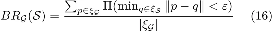
where ξSand ξGrespectively denote the union set of superpixel boundaries and the union set of groundtruth boundaries.The indicator function Π checks if the nearest pixel is withinεdistance.Here we follow Refs.[17,21]and setε=2 in our experiment.The boundary recall curves for different methods are plotted in Fig.5(a).One can easily observe that our FLIC method outperforms all other methods.

4.3.2 Undersegment error

The undersegment error(UE)[28]reflects the extent to which superpixels do not exactly overlap the ground-truth segmentation.As for BR,UE also reflects boundary adherence,but UE uses segmentation regions instead of boundaries in the measurement.Mathematically,UE can be computed by

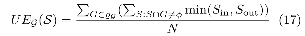
where ϱSis the union set of superpixels,ϱGis the union set of the segments of the ground-truth,Sindenotes the overlap between superpixelSand groundtruth segmentG,andSoutdenotes the rest of the superpixelS.As shown in Fig.5(b),our results are nearly the same as those of the best approach ERS[16],while our method is significantly faster.

4.3.3 Achievable segmentation accuracy

Achievable segmentation accuracy (ASA)[16]gives the highest accuracy achievable for object segmentation that utilizes superpixels as units.As for UE,ASA utilizes segments instead of boundaries.It can be computed by

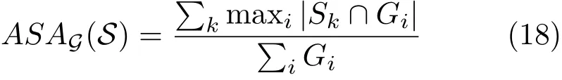
whereSkrepresents the superpixel andGirepresents the ground-truth segment. A better superpixel segmentation willhave a largerASA value.Figure 5(c)shows that,compared to the ERS method[16],the quality of results provided by our approach is competitive,and our method achieves the best trade-offbetween quality and speed.

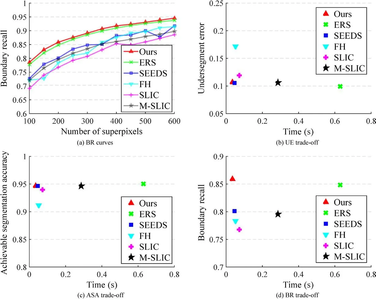
Fig.5 Comparisons between state-of-the-art methods and our approach on the BSDS500 benchmark.In(b)-(d),Kis fixed to 200 for the best trade-offbetween result quality and speed.In terms of boundary recall,our strategy significantly outperforms methods that take similar time.Furthermore,competitive results are also achieved compared to slower methods(e.g.,the state-of-the-art ERS method[16])according to all evaluation metrics,but at an order of magnitude faster speed.

4.3.4 Time

Similar to SLIC,our method hasO(N)time complexity.Speed is one of the most important issues for using superpixels as elementary units.Many approaches are limited by their speeds,such as SSS[19]and ERS[16].As shown in Fig.5,the average time taken by our FLIC method using two iterations to process an image is 0.035 s,while the time needed by ERS,Manifold SLIC,SLIC,and FH is 0.625 s,0.281 s,0.072 s,and 0.047 s,respectively.FLIC has the lowest time cost of all these methods and is nearly 20 times faster than ERS whilst providing comparable result quality.

4.3.5 Visual results and analysis

Figure 6 show several superpixel segmentation results using different algorithms. It can be seen that our approach is more sensitive to image boundaries,especially when there is poor contrast between the foreground and background.Compared to the SLIC method,our approach follows boundaries very well and runs twice as quickly.Compared to the ERS method,our superpixels are much more regular and the mean execution speed of our approach is 20 times greater.

The above facts and Fig.5 show that our approach achieves an excellent compromise between boundary adherence,compactness,and time.

4.4 Comparison using Pascal Context dataset

Additional,We evaluate the over-segmentation methods on Pascal Context dataset,which is larger and more realistic.We use the same metrics to evaluate the over-segmentation method.

4.4.1 Boundary recall

The boundary recall curves for different methods are plotted in Fig.7(a).We can see that almost all over-segmentation methods achieve quite high recall values.Our method is no longer the best but still achieves competitive performance.Figure 7(d)shows that our method achieves 0.974 in terms of boundary recall while the state-of-the-art method M-SLIC[21]achieves 0.978.However,our method runs ten times faster than M-SLIC.We think this difference may be because that there are fewer edges in the ground-truth in the Pascal Context dataset.

4.4.2 Undersegment error

Figure 7(b)shows that our results are nearly the same as those of the best approach,SEEDS[15],but run faster.

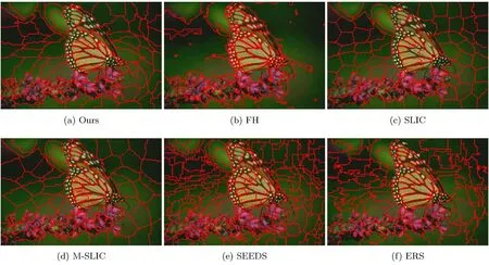
Fig.6 Visual comparison of superpixel segmentation results using various algorithms,with 100 superpixels andm=10.Our approach follows boundaries very well and at the same time produces compact superpixels.

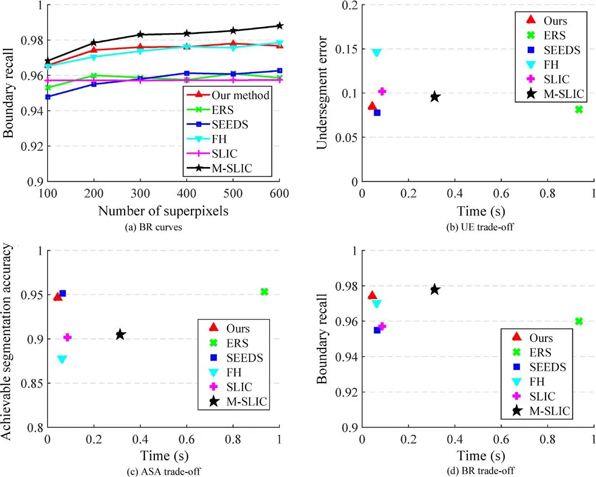
Fig.7 Comparisons between state-of-the-art methods and our approach on the Pascal Context dataset.Due to the simplicity of this dataset,almost all over-segmentation methods yield good boundary recall.The proposed method achieves a competitive trade-offon this dataset.

4.4.3 Achievable segmentation accuracy

Figure 7(c)shows that,compared to other oversegmentation methods,ourapproach provides competitive result quality,giving the best trade-offbetween quality and time.

4.4.4 Time

The size of images in the BSDS dataset is fixed,either 480×320 or 320× 480,while in the Pascal Context dataset,the image size is arbitrary.Figure 7 shows that our proposed method still takes least time amongst all over-segmentation methods.

4.5 Algorithm analysis

4.5.1 Efficacy of back-and-forth traversal

As shown in Fig.2,we adopt a back-and-forth traversal order to scan the whole enclosing bounding box for each superpixel.Actually,using two forward scans can also perform very well for our method.Figure 8 provides a quantitative comparison between two strategies:using four iterations of purely forward scanning,and using the proposed back-and-forth scan order twice(which also results in four iterations).The blue line indicates results using normal forward scan order while the red line indicates results using our method.The red curve significantly outperforms the blue curve while taking similar time:our back-andforth scan order considers more information about the regions outside the bounding box,leading to more reliable boundaries.

4.5.2 Role of spatial distance weight

Figure 9(a)shows that,unlike for SLIC[17],the BR curve monotonically decreases with respect to the spatial distance weightmin our approach.This is because in our method,local region continuity is mostly ensured by the active search algorithm,and color boundaries are less well preserved for largerm.On the other hand,smallmresults in less regular superpixels,so we choosem=5 for our comparison with previous works.Superpixels are normally used as a first step in vision tasks and these vision tasks often favor superpixel methods with good boundaries.Our approach allows users to select a reasonable value formaccording to their specific requirements.In any case,our overall performance is significantly better for all m values.

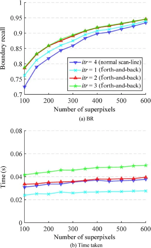
Fig.8 Partial sensitivity analysis for standard evaluation metrics and time taken.

4.5.3 Convergence rate

FLIC significantly accelerates the evolution so that we only need a few iterations before convergence.We compare the result quality for different numbers of iterations using the Berkeley benchmark.It can be easily seen from Fig.9(b)that our algorithm quickly converges after two iterations and further iterations only bring marginal benefits to the results.For example,whenKis set to 200,the boundary recall of the superpixels with only one iteration is 0.835;after two iterations it is 0.859 and after three iterations it is 0.860.The undersegment error values are 0.115,0.108,and 0.107,respectively,while the achievable segmentation accuracy values are 0.941,0.945,and 0.946,respectively.As can be seen in Fig.9(b),our algorithm not only converges much more quickly than SLIC(which requires ten iterations to converge),but also obtains better quality results.

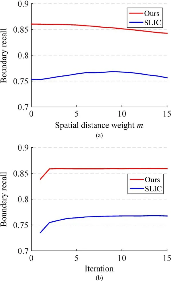
Fig.9 (a)BR-mcurves;mis the spatial distance weight in Eq.(1).Our results are far better than those from SLIC for all values ofm.(b)BR-iteration curves.Our method converges within 2 iterations,much fewer than SLIC.

4.5.4 Role of joint assignment and update

Our algorithm jointly performs the assignment and update steps. Figure 10 show the convergence rates for both our joint approach and for separately performing assignment and update steps.Clearly,our joint approach converges very quickly as only two iterations are needed,while the separate approach needs another two iterations to reach the same BR value.This demonstrates that our joint approach is efficient while having no negative effect on the final results.

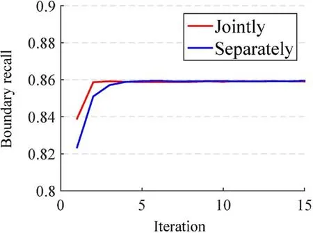
Fig.10 Comparison of convergence rate for joint and separate assignment and update steps.

4.5.5 Size of neighborhoods

In our method,the label of the current pixel relies on its four neighboring pixels.Using eight neighborhoods is also plausible,as more neighbors should definitely further more useful information.In Table 1,we briefly compare the results for these two approaches.As might be expected,larger neighborhoods lead to an increase in result quality but at the cost of reducing speed.In real applications,users can select either approach to suit their own requirements.

4.5.6 Traversal order

In our approach,we adopt the same traversal order as used in PatchMatch[23].Actually,there are many other possible traversal orders.Below we list a few simple ones:

·In PatchMatch,the horizontal axis is the major axis.Instead,we could first scan the vertical axis:forward scan first from top to bottom and then from left to right.Backward scan first from bottom to top and then from right to left.

·In PatchMatch,superpixels are scanned from the top left corner to the right bottom corner.Instead we may scan the superpixels from right bottom to top left.

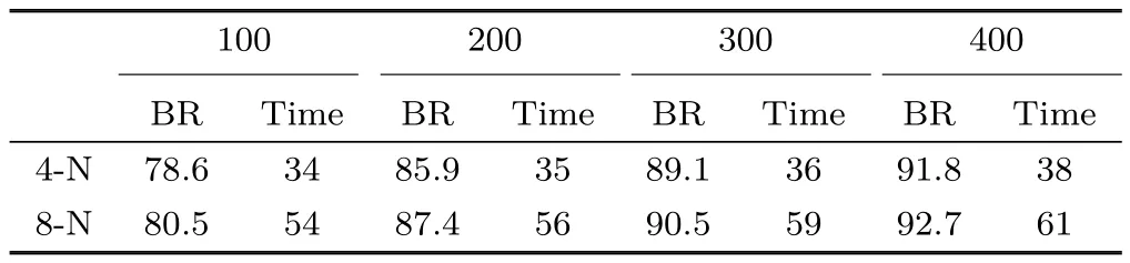
Table 1 Boundary recall versus time for 4-neighborhoods and 8-neighborhoods with different superpixel counts:100,200,300,400

· We also could combine the horizontal and vertical scans: first adopt the default traversal method,a horizontal scan,and then use a vertical scan,and so on.In our setting,we set the number of iterations to ten,with five horizontal and five vertical scans.

We compare results using different traversal orders in Table 2.The default traversal order achieves the best results amongst all possible traversal orders,but the difference is not great.In addition,the default traversal order is most straightforward to implement,hence we adopt it,as does PatchMatch[23].

4.5.7 Superpixel processing order

We further compared the results with and without sorting superpixels according to their entropies.If we process the superpixels in descending order of entropy,we get the results mentioned in previous experiments,with a boundary recall value of 85.9.However,the boundary recall is 84.8 if we process the superpixels according to their spatial order.As we can see,we get a minor improvement by sorting.

4.5.8 Qualitative results

Figure 11 shows some segmentation results for the BSDS dataset produced by our approach withm=20 and the number of superpixels set to 1000,400,and 200,respectively.It is seen that,in each case,the edges of the resulting superpixels are always very close to the boundaries.This is especially obvious in the first and third images.We also show some segmentation results for different values ofmin Fig.12.Whenmis smaller,for example 10,the shapes of the resulting superpixels become less regular.Whenmis larger,for example 30,the resulting superpixels become more compact.

In Figs.13 and 14 we show segmentation results for the Pascal Context dataset.Most images in the Pascal Context dataset come from real scenes,andare more complex than those in the BSDS dataset.As a result,the segmentation results are more cluttered.

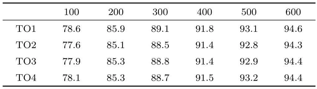
Table 2 Boundary recall for different traversal orders. TO1 represents the default traversal order which is first from left to right and then from top to bottom.TO2 represents traversing the pixels in a superpixel first from top to bottom and then from left to right.TO3 represents traversing the pixels first from right to left and then from bottom to top.TO4 represents the combined scheme

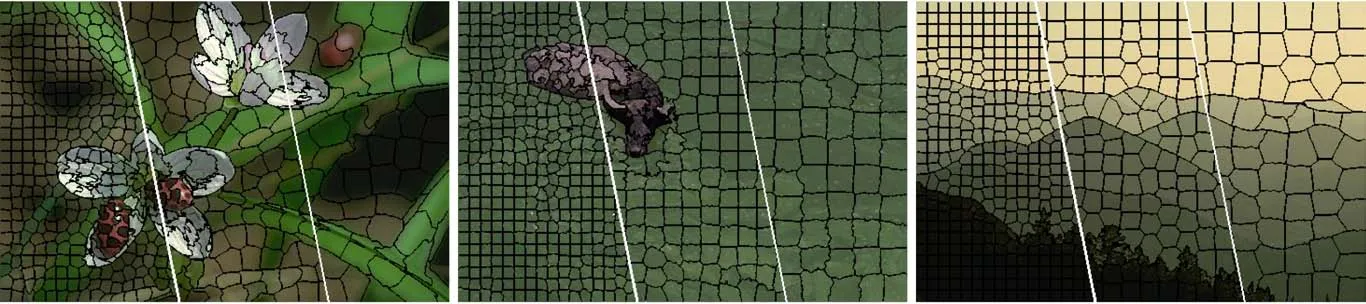
Fig.11 Images from the Pascal Context dataset segmented by our approach withm=20 and the number of superpixels set to 1000,400,and 200,respectively.The resulting superpixels follow region boundaries very well.

Fig.12 Images from the BSDS dataset segmented by our proposed approach withm=10,20,and 30,respectively.Whenmis smaller,the superpixels follow boundaries well.When m is larger,the superpixels are more compact.

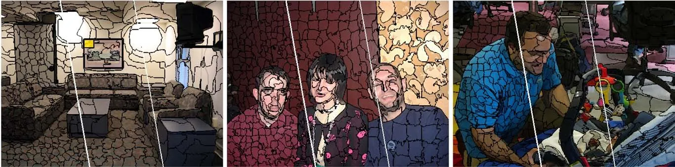
Fig.13 Images from the BSDS dataset segmented by our approach withm=20 and the number of superpixels set to 1000,400,and 200,respectively.The resulting superpixels follow region boundaries very well.

Fig.14 Images from the Pascal Context dataset segmented by our proposed approach withm=10,20,and 30,respectively.Whenmis smaller,the superpixels follow boundaries well.When m is larger,the superpixels are more compact.

5 Applications

In this section,we applied our method to a higher level application image segmentation problem[1].In hfs[1],image over-segmentation is used as an initial step:its results are taken as the input to the algorithm to generate a final segmentation result.In the original method,SLIC[17]is used to generate the image over-segmentation result.Here we simply replace SLIC with our proposed method and use the same image segmentation evaluation metric.However,we only use the optimal dataset scale(ODS)during training as the proposed method has few parameters.We use theF-measure of precision and recall on the whole dataset to evaluate the boundary performance;the following evaluation metrics are used to assess region performance:

· Variation of Information(VI),which measures the distance between ground-truth and the segmentation result.Lower VI is better.

· Probabilistic Rand Index(PRI),which measures the pairwise compatibility of element assignment between ground-truth and the proposed segmentation.A large value is better.

·Segmentation Covering (Covering), which measures the average overlap between groundtruth and the proposed segmentation.Again,a large value is better.

The results can be seen in Table 3.The segmentation results are closer when the number of superpixels is large,e.g.,1000 or 2000:as the number of superpixels increases,the quality of different over-segmentation methods becomes closer.When the number of superpixels is small,e.g.,100,segmentation results usingFLIC as the initial step perform better than those using SLIC.Hence,it is reasonable to say that our method is better than SLIC in practical applications.

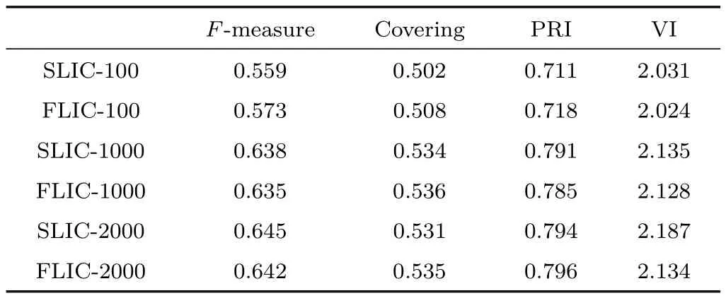
Table 3 Comparison of segmentation results generated by SLIC and FLIC for different numbers of superpixels.E.g.,SLIC-100 indicates use of SLIC to generate 100 superpixels which were then input to a downstream algorithm to achieve the final segmentation result

6 Conclusions

This paper has presented a novel algorithm using active search,which is able to improve the result quality and significantly reduce the time taken when producing superpixels to over-segment an image.Taking advantage of local continuity,our algorithm provides results with good boundary sensitivity even for complex and low contrast images.Moreover,it is able to converge in only two iterations,making it faster than previous methods,providing result quality comparable to the state-of-the-art ERS method in 1/20th of the time.We have used various evaluation metrics on the Berkeley segmentation benchmark dataset to demonstrate the speed and high quality results of our approach.

Acknowledgements

This research was sponsored by National Natural Science Foundation of China(Nos.61620106008 and 61572264),Huawei Innovation Research Program(HIRP),and IBM Global SUR Award.