The 3D Non-isentropic Compressible Euler Equations with Damping in a Bounded Domain∗

Yinghui ZHANG Guochun WU

1 Introduction

With damping,the three-dimensional compressible Euler equations for non-isentropic flows have the following form:

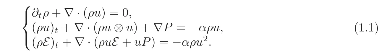
Such a system occurs in the mathematical modeling of compressible flow through a porous medium.Here ρ,u=(u1,u2,u3)tand P represent the density,the velocity and the pressure respectively.The total energy E=+e,where e is the internal energy.The constant α>0 models friction.In this paper,we will consider only polytropic fluids,so that the equations of state for the fluid are given by

where θ is the absolute temperature.The constants R>0 and γ >1 denote the gas constant and the adiabatic exponent,respectively.

For the isentropic flow,namely S=const.,(1.1)takes the form

The 1D version of(1.3)with various initial and initial-boundary conditions has been studied intensively during the past decades,both classical and weak solutions have been constructed,and the long time behaviors of different solutions have been investigated.There are extensive literatures for both the Cauchy problem and the initial-boundary value problem,and the readers are referred to[2,8–10,13,15-24,26–27,36,39,41–42]and references therein.For the multi-dimension problem to the isentropic system(1.3),Wang and Yang[34]proved the global existence and asymptotic behavior to the Cauchy problem for the isentropic system(1.3)by the Green function method.Sideris,Thomases and Wang[31]showed that the damping term prevented the development of singularities for small amplitude classical solutions in threedimensional space,using an equivalent reformulation of the Cauchy problem to obtain effective energy estimates.Pan and Zhao[29]investigated the global existence and asymptotic behavior to the initial boundary value problem for the isentropic system(1.3)by energy method.Fang and Xu[7]studied the existence and asymptotic behavior of C1solutions on the framework of Besov space.The optimal convergence rates were recently obtained by Tan and Wu[32].

For the adiabatic flow,namely S?=const.,much less is known even for the one-dimensional case.The global existence of smooth solution to the Cauchy problem for 1D version of(1.1)has been proved in[14,40]for small initial data.The large time behavior of these solutions is known only for some particular initial data(see[11,25]).For the initial boundary value problem,the readers are referred for instance to[12,28]and references therein.

From the physical point of view,the 3D model(1.1)describes more realistic phenomena.Also the 3D compressible non-isentropic Euler equations carry some unique features,such as the effect of vorticity,which are totally absent in the 1D case and make the problem more challenging in mathematics.The system(1.1)and the time-asymptotic behavior of the solution are of great importance and are much less understood than its 1D companion.Recently,the authors in[35,37]studied the global existence and asymptotic behavior of classic solutions to the Cauchy problem and the period boundary problem to the system(1.1)respectively.To our knowledge,there is no work on the global existence and asymptotic behavior of classical solution for the initial boundary value problem to the system(1.1).The main motivation of this article is to give a positive answer to this problem.

To begin with,we note the fact that all thermodynamics variables ρ,θ,e,P as well as the entropy S can be represented by functions of any two of them.To overcome the difficulties arising from non-isentropic,we rewrite the system(1.1).We take the two variables to be P and S,then the equation of state is replaced by

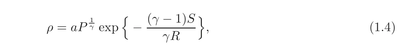
where a>0 is a constant.Under the aforementioned assumptions,we can rewrite the system(1.1)in terms of(P,u,S)as follows:

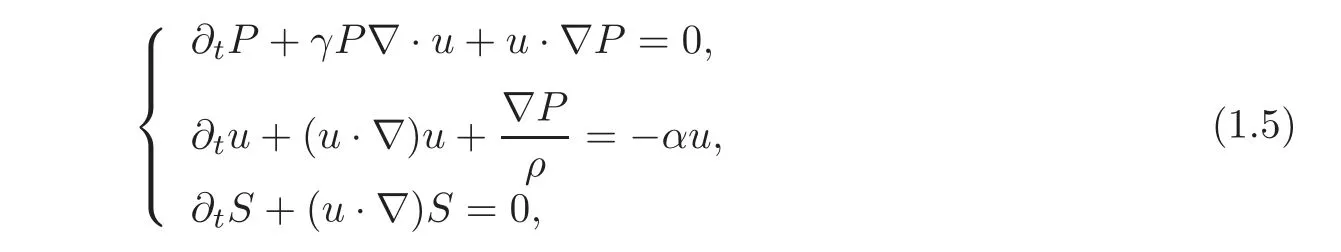
where ρ = ρ(P,S)is given by(1.4).It should be mentioned that(1.5)is a hyperbolic system,while the dissipation property comes from the damping term.In this paper,we consider the initial boundary value problem for(1.5)with the following initial and boundary conditions:

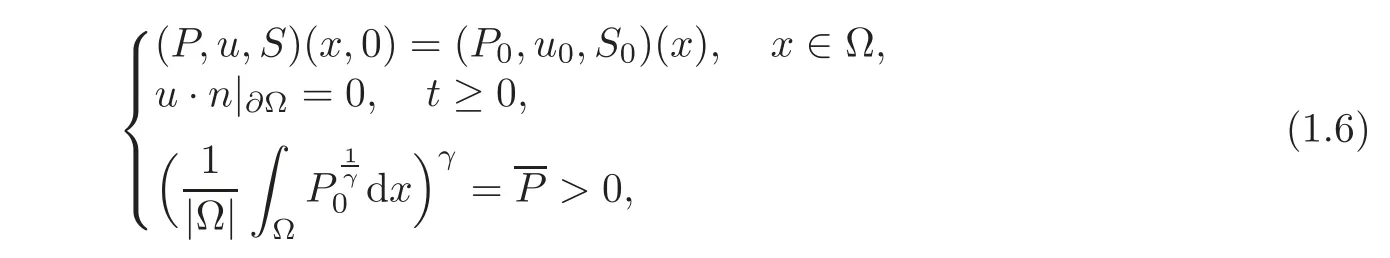
where Ω ⊂ R3is a bounded domain with smooth boundary ∂Ω,n is the unit outward normal vector on the boundary Ω and the last condition is imposed to avoid the trivial case,ρ ≡ 0.

Before stating the main results,let us introduce some notations for the use throughout this paper.C denotes some positive constant.The norms in the Sobolev spaces Hm(Ω)and Wm,q(Ω)are denoted respectively by?·?mand?·?m,qfor m ≥ 0 and q≥ 1.In particular,for m=0 we will simply use?·?and?·?Lq.?(a,b,c)?mdenotes?a?m+?b?m+?c?m.The energy space under consideration is

equipped with norm

for any F ∈ Xk([0,T],Ω)and t∈ [0,T].Moreover,we use?·,·?to denote the inner product in L2(Ω).Finally,

and for any integer l≥ 0,∇lf denotes all derivatives of order l of the function f.And for multi-indices α and β

we use

andwhere β ≤ α.

Now,we are ready to state the main results.

Theorem 1.1Assume that the initial data satisfy the compatibility condition,i.e.,n|Ω=0,0 ≤ l≤ 3,where(0)·=0 is the l-th time derivative at t=0 of any solution of(1.5)–(1.6),as calculated from(1.5)to yield an expression in terms of P0,u0and S0,andis sufficiently small.Then the initial boundary value problem(1.5)–(1.6)admits a unique solution(P,u,S)globally in time with P>0,satisfying

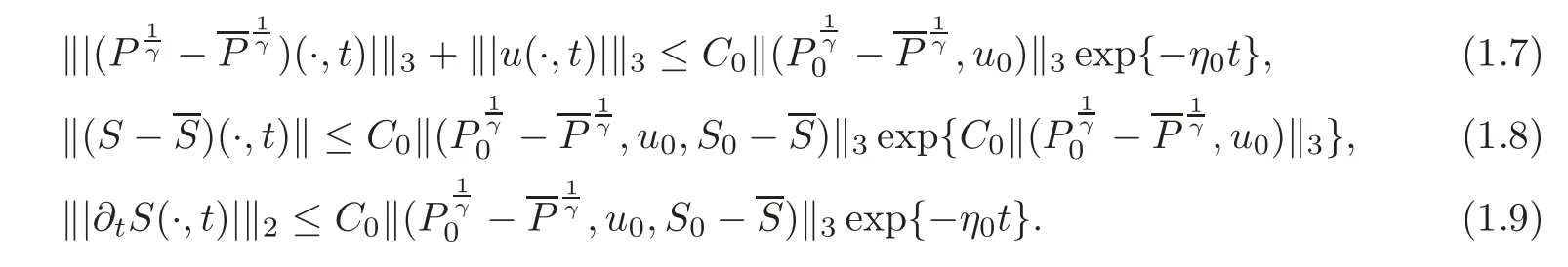
Moreover,there exist positive constants C0and η0,which are independent of t,such that for any t≥0,it holds

Remark 1.1The methods of this paper can be applied to study the global existence and asymptotic behavior for the initial boundary value problem to the 3D compressible nonisentropic Navier-Stokes equations without heat conductivity(see[3])and the 3D viscous liquidgas two phase flow model(see[38]).

Remark 1.2By applying the similar idea of[38],we can also prove that Theorem 1.1 still holds under only the smallness assumption on H2-norm of the initial data.

Now,we sketch the main idea of the proof and explain some of the main difficulties and techniques involved in the process.First,due to non-isentropic,we can not use the methods of[29,30–32,34]where the isentropic system(1.2)has been studied.To overcome the difficulties for the appearance of the non-isentropic term,as in[3,38],we first rewrite the system(1.1)into(1.5).However,we can not work directly on the system of the variables(P,u,S)as in[3,38].Indeed,on one hand,the integralis in general not zero since the variable P is not conservative.On the other hand,by noting the dissipation structure of(1.5),it is clear that there is no dissipation estimate for L2-norm of the variable P.Therefore,it seems impossible to get the exponential decay estimate on?P?by the Poincaré inequality and the Gronwall’s inequality as in[29].The key idea here is that instead of the variables(P,u,S),we study the system of the variables(ω,u,S)with(see(2.2)–(2.3)for details).One of main observations in this article is that the dissipative variables ω and u satisfy the first and second equations of(2.2)whose linear parts possess the same structure as that of the compressible isentropic Euler equations with damping(1.2),while the non-dissipative variable S satisfies the homogeneous transport equation the third equation of(2.2).Then,in order to obtain a priori estimates of solutions to(2.2)–(2.3),we can apply the similar energy method as in[3–5,29,33,37–38]to the first two equations of(2.2)to obtain the uniform bound of(ω,u)under the assumption that?(ω,u,S)?3is sufficiently small,see Lemmas 3.1–3.2 in Section 3.With these in hand,the variables(w,u)can be shown to converge exponentially to zero from the Poincaré inequality and Gronwall’s inequality.It is worth mentioning that the crucial part of the proof is to obtain a Lyapunov-type energy inequality(see(3.37)).Then,the bound of S will be derived by the exponential decay estimates on(w,u)and the Gronwall’s inequality.Second,due to the slip boundary condition,the classical energy estimates can not be applied directly to spatial derivatives.As in[29],the main idea is to get the key estimates of∇u by∇×u and∇·u,see Lemma 3.2 below.Using the special structure of(2.2)together with an induction on the number of spatial derivatives,the estimate of total energy is reduced to those for the vorticity and temporal derivatives.And the proof is completed by showing that(1.7)is true for the vorticity and temporal derivatives.

The plan of the rest of this paper is as follows.In Section 2,we reformulate the original system to get a quasi-linear symmetric hyperbolic system and give some basic facts that will be used in this paper together with the local existence result.In Section 3,we prove Theorem 1.1 by delicate energy estimates.

2 Reformulation and Local Existence

In this section,we are going to reformulate the initial-boundary value problem(1.5)–(1.6).First we reformulate(1.5)to get a symmetric hyperbolic system.Introducing the nonlinear transformationwe get from the original system(1.5)that

Denotingwithwe get the desired symmetric system for the perturbation(w,u,s)

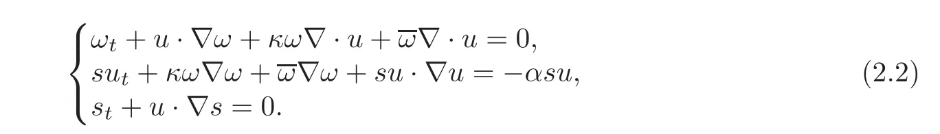
The initial and boundary conditions become

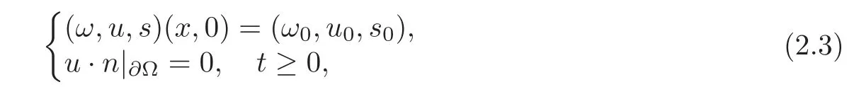
with

Before giving the proof of Theorem 1.1,we state the local existence result for the system(2.2)–(2.3),which can be established using the arguments in[3,26–27].

Proposition 2.1(Local Existence)Letbe fixed and suppose thatare such thatand satisfy the compatibility condition,i.e.,·n|Ω=0,0 ≤ l ≤ 3.Then there exists a positive constant ε0such that ifthen there exists a positive constant T0depending on ε0such that the initial-boundary value problem(2.2)–(2.3)admits a unique solution(ω,u,s − u) ∈which satisfies

and

To prove global existence of a smooth solution with small initial data,it suffices to establish global a priori estimate of the solution.

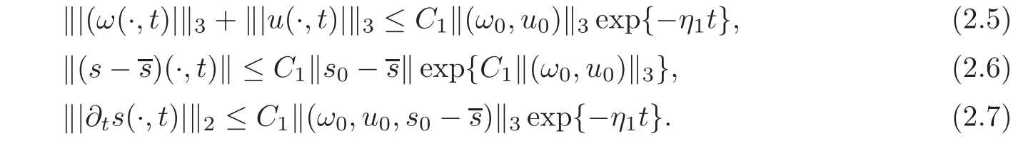
Proposition 2.2(A Priori Estimate) Let∈ H3(Ω)and suppose that the initial-boundary value problem(2.2)–(2.3)has a solutionX3([0,T],Ω)for given T>0.Then there exist a small positive constant ε1(≤ ε0)and two positive constants C1and η1,which are independent of T,such that if then for any t∈[0,T],it holds that

Proof of Theorem 1.1Choose ε2,C1and η1such thatC1=C0and η1= η0.Then the local solution of(2.2)–(2.3)can be continued globally in time,provided that the smallness conditionis satisfied.In fact,we haveTherefore,by Proposition 2.1,there is a positive constant T1=T1(ε1)such that a solution exists on[0,T1]and satisfiesfor t∈ [0,T1].Hence we can apply Proposition 2.2 with T=T1to get?(ω,u,s−Therefore,we can apply Proposition 2.1 by taking t=T1as the new initial time.Then we have a solution on[T1,2T1]with the estimate?(ω,u,s−for t ∈ [T1,2T1].Thereforeholds on[0,2T1].Hence Proposition 2.2 again gives the estimates(2.5)–(2.7)for t∈ [0,2T1].In the same way we can extend the solution to the interval[0,nT1]successively,n=1,2,···,and get a global solution.The estimates(1.7)–(1.9)is a consequence of(2.5)–(2.7).This completes the proof of Theorem 1.1.

The proof of Proposition 2.2 is based on several steps of careful energy estimates which are stated as a sequence of lemmas in Section 3.

3 Global Existence and Large Time Behavior

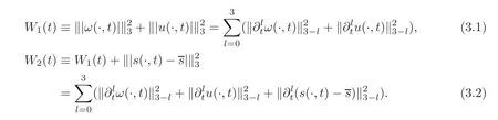
In this section,we devote ourselves to prove Proposition 2.2.For convenience,we let

Throughout this section,we suppose that the initial-boundary value problem(2.2)–(2.3)has a solution(ω,u,s−)in the spacewith some T ∈ (0,+∞],and the inequality(2.4)holds.We also omit the variable t of all functions in the proof of different lemmas in this section for simplicity.

In what follows,a series of lemmas on the energy estimates are given.First we recall some inequalities of Sobolev type(see[6]).

Lemma 3.1Let Ω be any bounded domain in R3with smooth boundary.Then it holds:

(i)?f?L∞(Ω)≤ C?f?H2(Ω),

(ii)?f?Lq(Ω)≤ C?f?H1(Ω),2 ≤ q ≤ 6

for some constant C>0 depending only on Ω.

As in[29],the following lemma(see[1])plays an important role in our proofs,which gives the estimate of∇u by∇·u and∇×u.

Lemma 3.2Let u ∈ Hk(Ω)be a vector-valued function satisfying u ·n|Ω=0,where n is the unit outer normal of∂Ω.Then

for k ≥ 1,where constant C depends only on k and Ω.

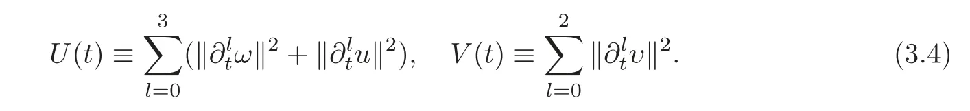
The next lemma is an application of Lemma 3.2,which is crucial to complete the proof of Proposition 2.2.Indeed,the lemma states that the bounds of spatial derivatives can be controlled by those of the temporal derivatives and the vorticity.Let υ =∇ ×u and define

Lemma 3.3Under the assumptions of Proposition 2.2,there exists a constant C2>0 which is independent of ε such that

ProofFrom the equation(2.2)2,we have

Using the smallness of W2(t),Lemma 3.1 and Cauchy-Schwarz inequality,we easily get

and

Taking time derivatives of(3.6)twice,after a tedious but direct computation,we also have

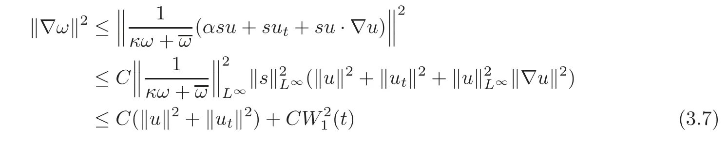
By using the first equation of(2.2),we have

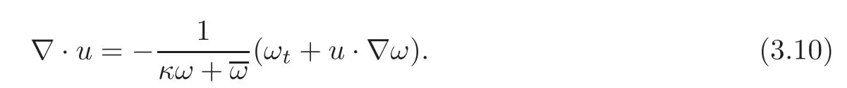
So,we can easily get

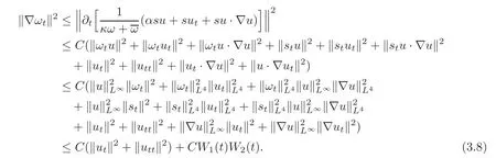
Using Lemma 3.2 with k=1 and(3.11),we obtain

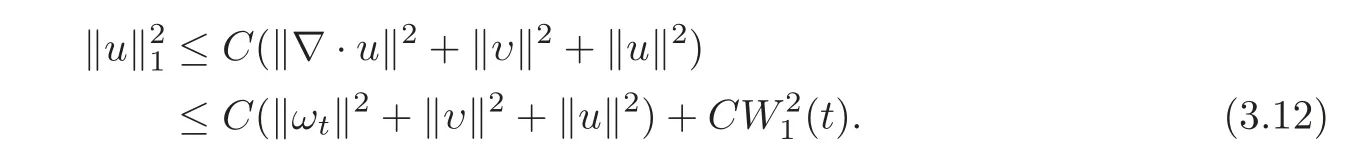
Next,we take time derivatives of(3.10).It is easy to see that every time derivative up to order two of∇·u can be bounded by U(t)+W1(t)W2(t).Furthermore,together with an induction on the number of spatial derivatives,the same is true for any derivative up to order two of∇·ω and∇·u.By applying Lemma 3.2 with k=1,2,3 respectively,we can deduce that

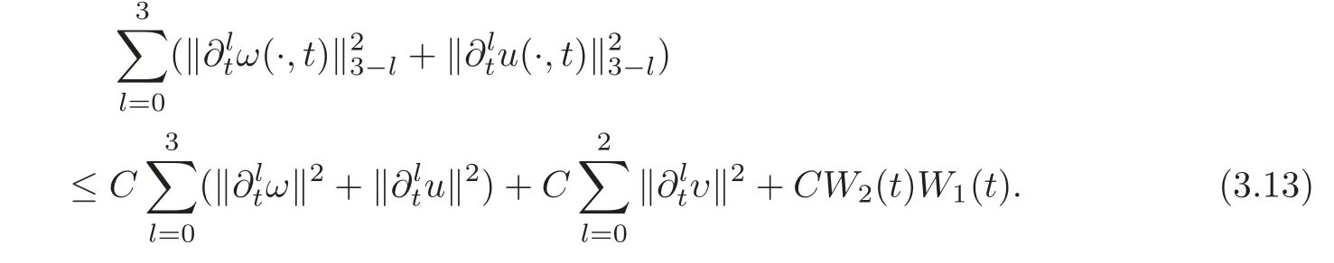
Since W2(t)is small,we prove(3.5).Therefore,the proof of Lemma 3.3 is completed.

Lemma 3.3 reduces the estimate of W(t)to those for U(t)and V(t).In the following,we will devote ourselves to deduce the estimates of U(t)and V(t).

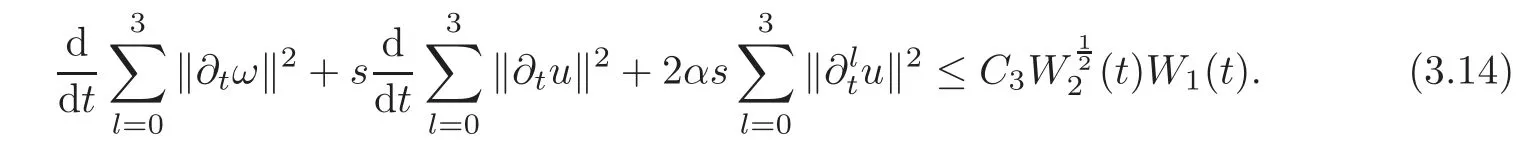
Lemma 3.4Under the assumptions of Proposition 2.2,there exists a constant C3>0 which is independent of ε such that

ProofIn the following,we will prove Lemma 3.4 by five steps.

Step 1Zero order estimate Multiplying the first and second equations of(2.2)by ω,u respectively and then integrating them over Ω,using the boundary condition u ·n|∂Ω=0,we have

From Lemma 3.1,H¨older’s inequality and Cauchy-Schwarz inequality,we have

Step 2First order estimate differentiating the first and second equations of(2.2)with respect to t once,multiplying the resultant equations by ωt,utrespectively,integrating over Ω and using the boundary conditionswith l=0,1,we have

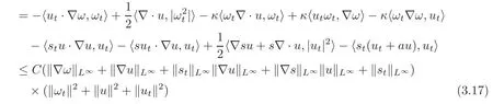
for some constant C>0.From Lemma 3.1,H¨older inequality and Cauchy-Schwarz inequality,we deduce that

Step 3Second order estimate Repeating the above procedure again for 2nd order time derivatives,we can get

for some constant C>0.By virtue of Lemma 3.1,H¨older inequality and Cauchy-Schwarz inequality,we have

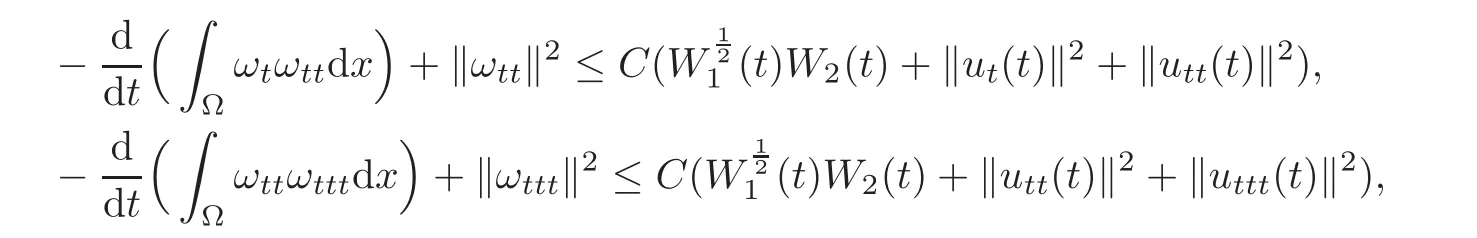
Step 4Third order estimate Repeating the above procedure again for 3rd order time derivatives,we get the following

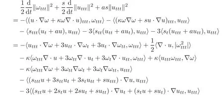
By virtue of Lemma 3.1,H¨older’s inequality and Cauchy-Schwarz inequality,we have

Bounds for the other terms are obtained in a similar way,we finally deduce

Since W2(t)is small,substituting the above two inequalities into(3.21),we finally obtain

Step 5Proof of Lemma 3.4 Putting(3.16),(3.18),(3.20)and(3.22)together gives(3.14).This completes the proof of Lemma 3.4.

Lemma 3.4 contains only the dissipation in velocity.In the next lemma,we will deduce the dissipation in pressure due to nonlinearity.

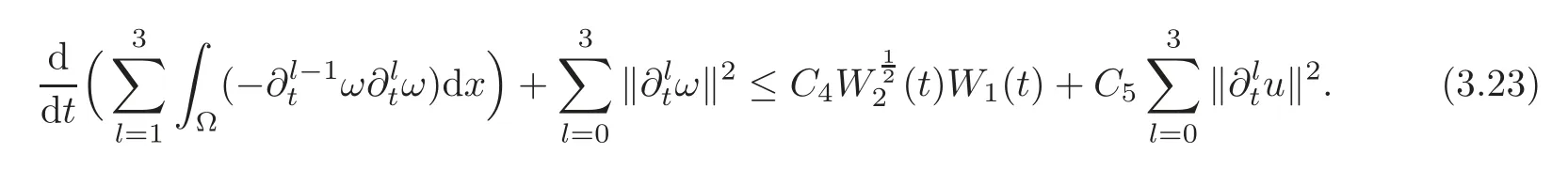
Lemma 3.5Under the assumptions of Proposition 2.2,there exist two positive constants C4,C5which are independent of ε such that

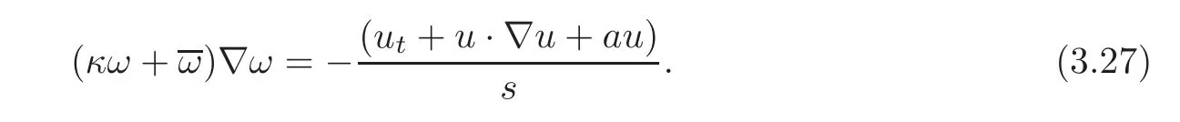
ProofFirst of all,we? n otice thatsatisfies the continuity equation,i.e.,which yieldsThis together with Poincaré’s inequality implies thatSince W2(t)is small,we can deduce thatis equivalent toandis equivalent tothus we haveBy using(3.7),we have

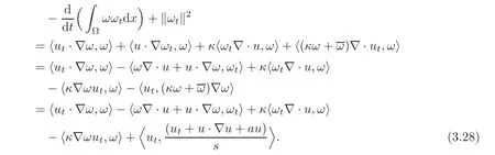
differentiating the first equation of(2.2)with respect to t,we get

Multiplying(3.25)by ω and integrating the resultant equation over Ω,we obtain

From the second equation of(2.2),we have

Substituting(3.27)into(3.26),using the boundary conditionswith l=0,1 and integrating by part,we have

Using the same idea in proof of Lemma 3.4,we have

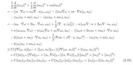
Repeating the above procedure again for 2nd and 3rd order time derivatives of(3.25),we have

which together with(3.24)and(3.29)implies(3.23).This completes the proof of Lemma 3.5.

Now,we are ready to combine Lemma 3.4 and Lemma 3.5 to deduce the total dissipation.To do this,we let D1>0 be a suitably large positive constant,and define

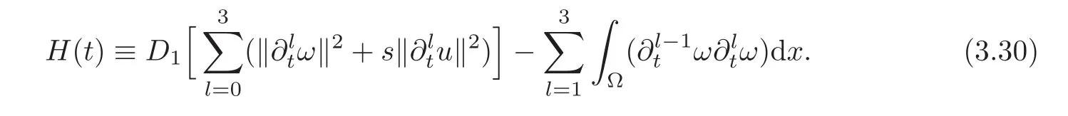
Since D1>0 is large enough andis sufficiently small,the function H(t)is equivalent to U(t).

Lemma 3.6Under the assumptions of Proposition 2.2,there exist two positive constants C6,C7which are independent of ε such that

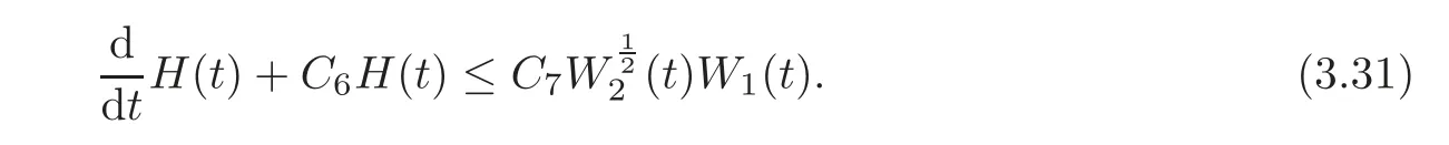
ProofD1×(3.14)+(3.23)yields

Since D1>0 is large andis small,we deduce(3.31)directly from(3.32).This completes the proof of lemma.

The last lemma is concerned with the dissipation in V(t)defined in(3.4).

Lemma 3.7Under the assumptions of Proposition 2.2,there exists a positive constant C8which is independent of ε such that

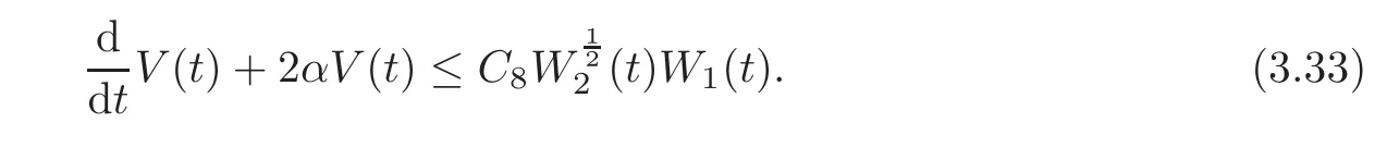
ProofTaking the curl of the second equation of(2.2),we get

Taking any mixed derivative of the above equation,we obtain

where α1,α2satisfyNoticing thatmultiplying the above equation byand integrating the resulting equation by using the boundary condition,together with the standard energy estimate used in deriving Lemmas 3.4–3.5,we deduce(3.33).This completes the proof of lemma.

Now we are in a position to prove Proposition 2.2.

Proof of Proposition 2.2If we define

then from Lemmas 3.6–3.7,there exist two positive constants C9,C10which are independent of ε such that

Moreover,since H1(t)is equivalent to U(t)+V(t),we have from Lemma 3.3 that

Since ε>0 is small,combining(3.37)and(3.38),we have that there exists a constant C11>0 such that

which yields the exponential decaying of H1(t).Since H1(t)is equivalent to U(t)+V(t),(2.5)follows from Lemma 3.3 immediately.Next,we prove(2.6).To do this,by multiplying the third equation of(2.2)by s −and integrating over Ω,using the boundary condition u ·n|∂Ω=0,we have

which yields(2.6).Finally,by symmetry,boundary conditions and some tedious but straightforward calculation,we have the energy estimates on the entropy:

thus we haveTaking the derivatives of the third equation of(2.2),we have

where|α1|+|α2|≤ 2.In fact,we first take|α1|=0,then we can easily prove that(3.40)is right.Taking an induction on α,we finally deduce(3.40)which gives(2.7).This completes the proof of Proposition 2.2.

AcknowledgementThe authors would like to thank the anonymous referees for their valuable suggestions and comments which have helped to improve the manuscript.

[1]Bourguignon,J.P.and Brezis,H.,Remarks on the Euler equation,J.Funct.Anal.,15,1975,341–363.

[2]Dafermos,C.M.,Can dissipation prevent the breaking of waves? Transactions of the Twenty-Sixth Conference of Army Mathematicians,187–198,ARO Rep.81,1,U.S.Army Res.Office,Research Triangle Park,N.C.,1981.

[3]Duan,R.J.and Ma,H.F.,Global existence and convergence rates for the 3-D compressible Navier-Stokes equations without heat conductivity,Indiana Univ.Math.J.,57(5),2008,2299–2319.

[4]Duan,R.J.,Liu,H.X.,Ukai,S.and Yang,T.,Optimal Lp−Lqconvergence rates for the compressible Navier-Stokes equations with potential force,J.differ.Equations,238,2007,220–233.

[5]Duan,R.J.,Ukai,S.,Yang,T.and Zhao,H.J.,Optimal convergence rate for compressible Navier-Stokes equations with potential force,Math.Models Methods Appl.Sci.,17,2007,737–758.

[6]Evans,L.C.,Partial differential Equations,Amer.Math.Soc.,Providence,1998.

[7]Fang,D.Y.and Xu,J.,Existence and asymptotic behavior of C1solutions to the multi-dimensional compressible Euler equations with damping,Nonlinear Anal.,70,2009,244–261.

[8]Hsiao,L.,Quasilinear Hyperbolic Systems and Dissipative Mechanisms,Singapore,World Scientific,1998.

[9]Hsiao,L.and Liu,T.P.,Convergence to nonlinear diffusion waves for solutions of a system of hyperbolic conservation laws with damping,Comm.Math.Phys.,143,1992,599–605.

[10]Hsiao,L.and Liu,T.P.,Nonlinear diffusive phenomena of nonlinear hyperbolic systems,Chin.Ann.Math.Ser.B,14(1),1993,1–16.

[11]Hsiao,L.and Luo,T.,Nonlinear diffusive phenomena of solutions for the system of compressible adiabatic flow through porous media,J.differ.Equations,125,1996,329–365.

[12]Hsiao,L.and Pan,R.H.,Initial-boundary value problem for the system of compressible adiabatic flow through porous media,J.differ.Equations,159,1999,280–305.

[13]Hsiao,L.and Pan,R.H.,The damped p-system with boundary effects,Contemporary Mathematics,255,2000,109–123.

[14]Hsiao,L.and Serre,D.,Global existence of solutions for the system of compressible adiabatic flow through porous media,SIAM J.Math.Anal.,27,1996,70–77.

[15]Huang,F.M.,Marcati,P.and Pan,R.H.,Convergence to Barenblatt solution for the compressible Euler equations with damping and vacuum,Arch.Ration.Mech.Anal.,176,2005,1–24.

[16]Huang,F.M.and Pan,R.H.,Asymptotic behavior of the solutions to the damped compressible Euler equations with vacuum,J.differ.Equations,220,2006,207–233.

[17]Huang,F.M.and Pan,R.H.,Convergence rate for compressible Euler equations with damping and vacuum,Arch.Ration.Mech.Anal.,166,2003,359–376.

[18]Jiang,M.N.,Ruan,L.Z.and Zhang,J.,Existence of global smooth solution to the initial boundary value problem for p-system with damping,Nonlinear Anal.,70(6),2009,2471–2479.

[19]Jiang,M.N.and Zhang,Y.H.,Existence and asymptotic behavior of global smooth solution for p-system with nonlinear damping and fixed boundary effect,Math.Meth.Appl.Sci.,37,2014,2585–2596.

[20]Jiang,M.N.and Zhu,C.J.,Convergence rates to nonlinear diffusion waves for p-system with nonlinear damping on quadrant,Discrete Contin.Dyn.Syst.,23(3),2009,887–918.

[21]Jiang,M.N.and Zhu,C.J.,Convergence to strong nonlinear diffusion waves for solutions to p-system with damping on quadrant,J.differ.Equations,246(1),2009,50–77.

[22]Liu,T.P.,Compressible flow with damping and vacuum,Japan J.Appl.Math.,13,1996,25–32.

[23]Marcati,P.and Milani,A.,The one-dimensional Darcy’s law as the limit of a compressible Euler flow,J.differ.Equations,84(1),1990,129–147.

[24]Marcati,P.and Rubino,B.,Hyperbolic to parabolic relaxation theory for quasilinear first order systems,J.differ.Equations,162(2),2000,359–399.

[25]Marcati,P.and Pan,R.H.,On the diffusive pro files for the system of compressible adiabatic flow through porous media,SIAM J.Math.Anal.,33,2001,790–826.

[26]Nishida,T.,Global solutions for an initial-boundary value problem of a quasilinear hyperbolic systems,Proc.Japan Acad.,44,1968,642–646.

[27]Nishida,T.,Nonlinear Hyperbolic Equations and Relates Topics in Fluid Dynamics,Publ.Math.D’Orsay,1978.

[28]Pan,R.H.,Boundary effects and large time behavior for the system of compressible adiabatic flow through porous media,Michigan Math.J.,49,2001,519–539.

[29]Pan,R.H.and Zhao,K.,The 3D compressible Euler equations with damping in a bounded domain,J.differ.Equations,246,2009,581–596.

[30]Schochet,S.,The compressible Euler equations in a bounded domain:Existence of solutions and the incompressible limit,Comm.Math.Phys.,104,1986,49–75.

[31]Sideris,T.C.,Thomases,B.and Wang,D.H.,Long time behavior of solutions to the 3D compressible Euler equations with damping,Comm.Partial differential Equations,28,2003,795–816.

[32]Tan,Z.and Wu,G.C.,Large time behavior of solutions for compressible Euler equations with damping in R3,J.differ.Equations,252(2),2012,1546–1561.

[33]Tan,Z.and Wang,H.Q.,Global existence and optimal decay rate for the strong solutions in H2to the 3-D compressible Navier-Stokes equations without heat conductivity,J.Math.Anal.Appl.,394(2),2012,571–580.

[34]Wang,W.and Yang,T.,The pointwise estimates of solutions for Euler equations with damping in multidimensions,J.differ.Equations,173,2001,410–450.

[35]Wu,G.C.,Tan,Z.and Huang,J.,Global existence and large time behavior for the system of compressible adiabatic flow through porous media in R3,J.differ.Equations,2553,2013,865–880.

[36]Zhang,Y.H.and Tan,Z.,Existence and asymptotic behavior of global smooth solution for p-system with damping and boundary effect,Nonlinear Anal.,72(5),2010,2499–2513.

[37]Zhang,Y.H.and Wu,G.C.,Global existence and asymptotic behavior for the 3d compressible nonisentropic Euler equations with damping,Acta Mathematica Sci.Ser.B,34(5),2014,424–434.

[38]Zhang,Y.H.and Zhu,C.J.,Global existence and optimal convergence rates for the strong solutions in H2to the 3D viscous liquid-gas two-phase flow model,J.differ.Equations,258(7),2015,2315–2338.

[39]Zhao,H.J.,Convergence to strong nonlinear diffusion waves for solutions of p-system with damping,J.differ.Equations,174,2001,200–236.

[40]Zheng,Y.,Global smooth solutions to the adiabatic gas dynamics system with dissipation terms,Chin.Ann.Math.Ser.A,17,1996,155–162(in Chinese).

[41]Zhu,C.J.,Convergence rates to nonlinear diffusion waves for weak entropy solutions to p-system with damping,Sci.China,Ser.A,46(4),2003,562–575.

[42]Zhu,C.J.and Jiang,M.N.,Lp-decay rates to nonlinear diffusion waves for p-system with nonlinear damping,Sci.China,Ser.A,49(6),2006,721–739.