The Third Initial-boundary Value Problem for a Class of Parabolic Monge-Ampre Equations∗

L BO-QIANGAND LI FENG-QUAN

(1.School of Mathematical Sciences,Dalian University of Technology,Dalian,

Liaoning,116024)

(2.College of Mathematics and Information Science,Nanchang Hangkong University, Nanchang,330063)

The Third Initial-boundary Value Problem for a Class of Parabolic Monge-Ampre Equations∗

(1.School of Mathematical Sciences,Dalian University of Technology,Dalian,

Liaoning,116024)

(2.College of Mathematics and Information Science,Nanchang Hangkong University, Nanchang,330063)

For the more general parabolic Monge-Ampre equations de fi ned by the operator F(D2u+σ(x)),the existence and uniqueness of the admissible solution to the third initial-boundary value problem for the equation are established.A new structure condition which is used to get a priori estimate is established.

parabolic Monge-Ampre equation,admissible solution,the third initialboundary value problem

1 Introduction and Statement of the Main Results

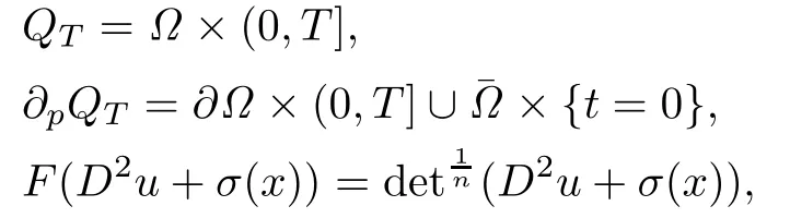
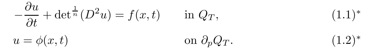
In this paper,we discuss the third initial-boundary value problem for parabolic Monge-Ampre equations

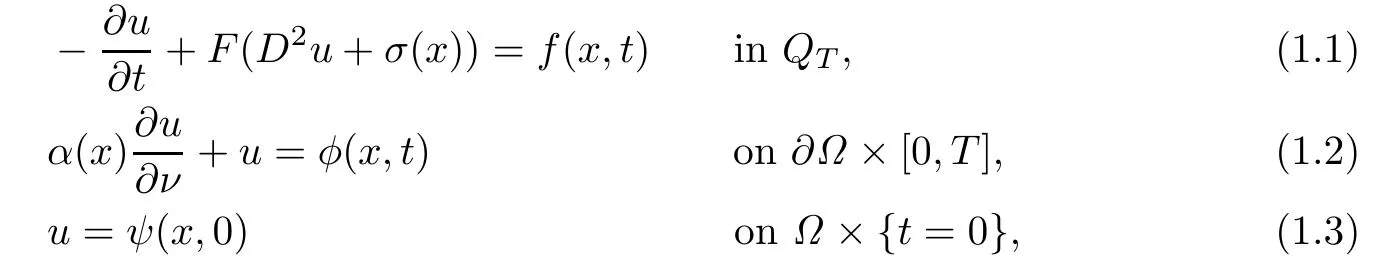
whereΩis a bounded uniformly convex domain inRn,

and

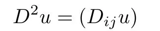
is the Hessian of u with respect to the variable x,ν is the unit exterior normal at(x,t)∈∂Ω×[0,T]to∂Ω,which has been extended on¯QTto be a properly smooth vector field independent of t,α(x)＞0 is properly smooth for all x∈ ¯Ω,σ(x)=(σij(x))is an n× n symmetric matrix with smooth components,f(x,t),φ(x,t),ψ(x,t)are given properly smooth functions and satisfy some necessary compatibility conditions.

The first initial-boundary value problem for a class of elliptic Monge-Ampre equations

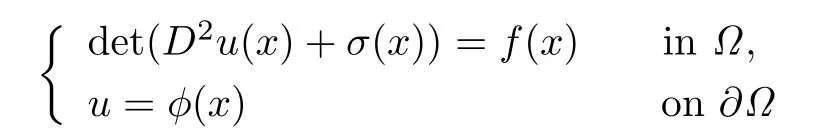
was firstly discussed by Ca ff arelliet al.[1]

Ivochkina and Ladyzhenskaya[2]studied the following first initial-boundary value problem for parabolic Monge-Ampre equations

They derived two structure conditions as follows:

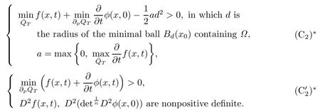
By(C2)∗or()∗,they obtained the existence and uniqueness of the solution.The third initial-boundary value problem for equation(1.1)∗was studied by Zhou and Lian[3].They also got two structure conditions similar to(C2)∗and()∗in[2].

Therefore,it is natural for us to consider the problem(1.1)–(1.3)as an extension of the result of[2–3].

De fi nition 1.1We say thatu(x,t)is an admissible function of(1.1)–(1.3)ifu(x,t)∈K, where

De fi nition 1.2We say thatu(x,t)is an admissible solution of(1.1)–(1.3)if an admissible functionu(x,t)satis fies(1.1)–(1.3).

Obviously,the equation(1.1)is of parabolic type for any admissible function u(x,t).

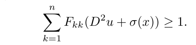
For any admissible solution,the following condition is necessary:

Following the idea of[2],we derive two structure conditions as follows:

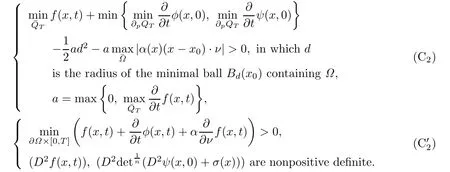
Especially,we drive a new type of structure condition

Our main result is as follows.

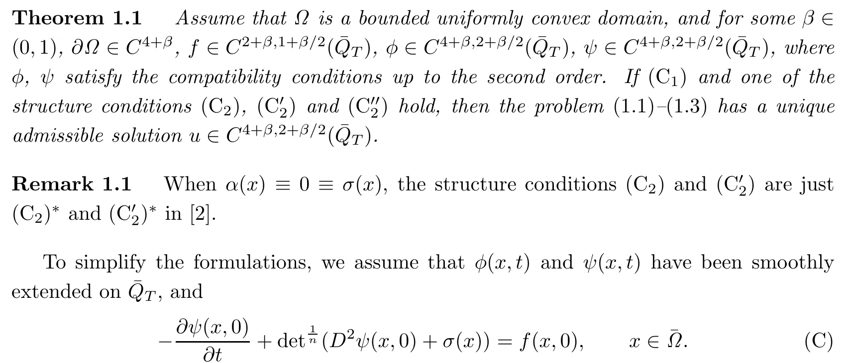
Similarly to the argument in[4],we use Weyl’s theorem(see[5])to overcome the difficulty coming from σ=σ(x)in(1.1).However,if σ=σ(x,t)in(1.1),then the difficulty in the process of deriving the structure conditions is so hard that we are not accomplished.

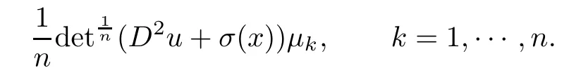
Lemma 1.1[5](Weyl’s Theorem)Assume thatAandBare all real symmetric matrices of ordern.Denote the eigenvalues ofA,B,A+Brespectively byλi(A),λi(B),λi(A+B),i=1,···,n.Suppose that these eigenvalues are arranged in increasing order,i.e.,forC=A,B,A+B,we have

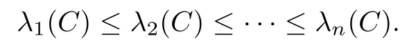
Then for eachk=1,2,···,n,it holds that

It is necessary to give some known results for further discussion.Denote

Then we have several lemmas as follows.

The structure of this paper is stated as follows:In Section 2,we show the existence and uniqueness of the admissible solution in Theorem 1.1 by using the method of continuity and comparison theorem.In Section 3,the generalized approach for deriving the structure conditions is presented,and the positive lower bound of F(D2u+σ(x))is obtained.In Section 4,a series of a priori estimates are established.

2 The Method of Continuity and Comparison Theorem

In order to get the existence of admissible solution in Theorem 1.1 by the method of continuity,we consider a family of problems with one parameter τ∈[0,1]as follows:

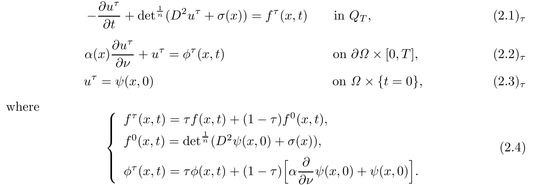
Obviously,for τ=1 the problem(2.1)τ–(2.3)τis just(1.1)–(1.3).

Remark 2.1If the assumptions of Theorem 1.1 hold,it is easy to find that the admissible solutions to problem(2.1)τ–(2.3)τsatisfy the compatibility condition up to order two uniformly with respect to τ by direct calculations.

Set

In order to prove the existence of admissible solution in Theorem 1.1 by the method of continuity,we only need to prove that S is nonempty,and also S is a relatively both open and closed set in[0,1].

Let τ=0.It is obvious that u0(x,t)≡ψ(x,0)is a solution of(2.1)τ–(2.3)τin V,i.e.,S is nonempty.

In order to show that S is a relatively open set in[0,1],we need the following lemma.Lemma 2.1[6]LetX1,X2and Σ be Banach spaces,andGbe a mapping from an open setUinX1×Σ intoX2.If there exists a(w0,τ0)∈Usatisfying

(1)G(w0,τ0)=0;

(2)Gis differentiable at(w0,τ0);

(3)Gw(w0,τ0)is invertible,

then there exists a neighborhoodNofτ0in Σ such that the equation

is solvable for eachτ∈Nwith the solutionw=wτ∈X1.

Actually,we can choose

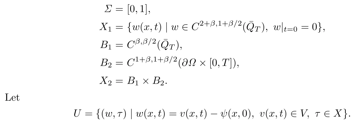
It is easy to prove that U is an open set in X1×Σ.

Set

Then G1and G2are mappings from the open set U into B1and B2respectively,and G is a mapping from U into X2.

Let w0∈U,τ0∈[0,1]be such that

It is easy to find that G is differentiable at(w0,τ0)if G1and G2are differentiable at(w0,τ0) with the Frchet derivative

Since G1is a linear parabolic operator and G2is an oblique derivative operator,by Theorem 5.3 of Chapter 7 in[7],we know that

is invertible.Therefore,by Lemma 2.1,there exists a neighborhood N ⊂[0,1]of τ0such that N⊂S.This proves that S is a relatively open set in[0,1].

In order to prove S is a relatively close set in[0,1],we need to establish the following a priori estimate.

Theorem 2.1If the assumptions of Theorem1.1hold,then there exist two positive constantsα∈(0,1)andCindependent ofτsuch that

holds for all solutionsuτof the problem(2.1)τ–(2.3)τ.

Thus we can prove that S is a relatively close set in[0,1]by Theorem 2.1 and Ascoli-Arzela lemma.It is easy to check that the data of(2.1)τand(1.1)have the same characters. So it suffices to establish the a priori estimate(2.5)for all admissible solutions u of(1.1).

To prove the uniqueness of the admissible solution in Theorem 1.1,we need the following comparison theorem.

Lemma 2.2[3]Assume that(aij(x,t))is a non-negative de finite matrix,u∈C2,1(QT)∩C1,0(),α(x)≥0for anyxon∂Ω,and

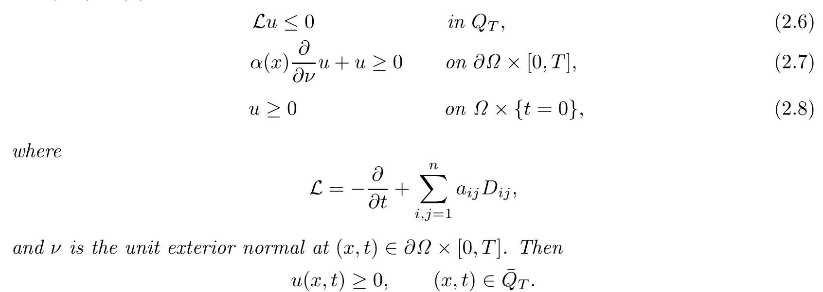
Theorem 2.2If the assumptions of Theorem1.1hold,then there exists at most one admissible solution of the problem(1.1)–(1.3).

Proof.If u1and u2are two admissible solutions of(1.1)–(1.3),then=u1−u2satis fies

3 A Positive Lower Bound Estimate of F(D2u(x,t)+σ(x))

For convenience of statements,we call a constant depending only on the data of the problem as a controllable constant.

The structure conditions(C2),(),()are used to estimate a positive lower bound of F(D2u(x,t)+σ(x)).From now on,we show a generalized approach for deriving these structure conditions.

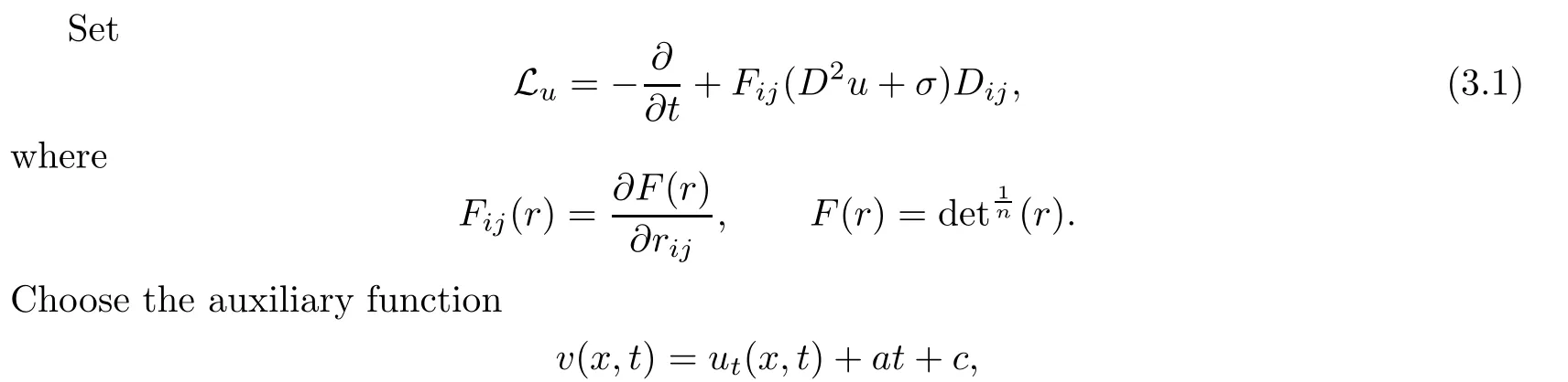
where u is an admissible solution of the problem(1.1)–(1.3),a≥0 and c are constants to be chosen.

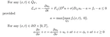
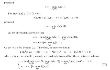
Thus we have the following theorem.

Theorem 3.1If the assumptions of Theorem1.1(except(C2)and(C′2))hold,then there exists a controllable positive constantγsuch thatF(D2u(x,t)+σ(x))has a positive lower bound,whereuis an admissible solution of the problem(1.1)–(1.3).

Remark 3.1We can get the structure condition(C2)by choosing the auxiliary function

where a≥0 and c are to be chosen,and x0is an arbitrary fixed point inΩ.

Remark 3.2We can get the structure condition()by choosing the auxiliary function

where c is to be chosen.

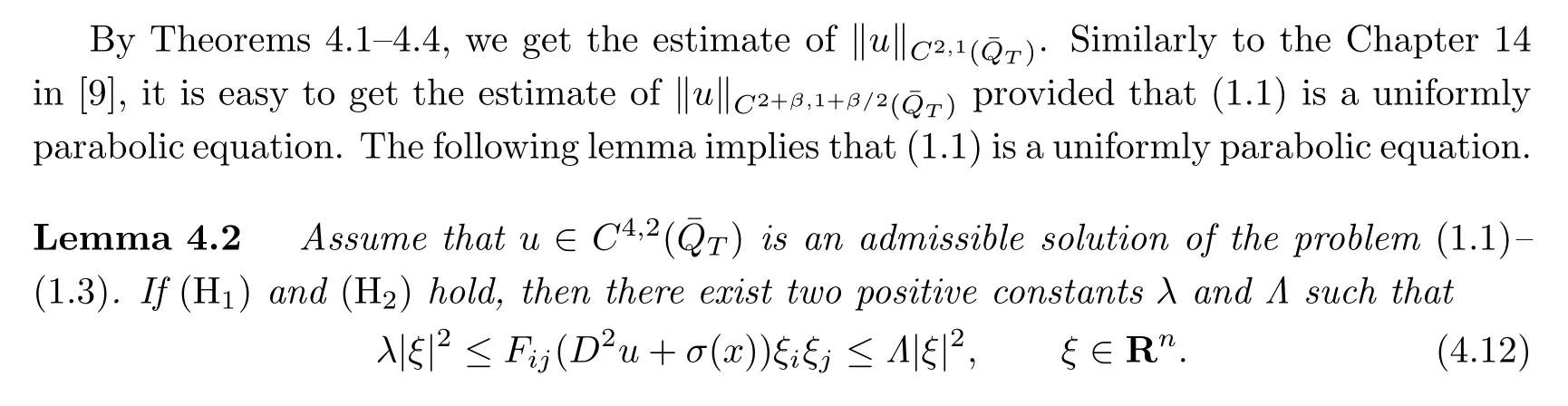
4 A Priori Estimate of kukC2+α,1+α/2()

Theorem 4.1If the assumptions of Theorem1.1hold,then there exists a controllable constantC0＞0such that

holds for all admissible solutionsuof the problem(1.1)–(1.3).

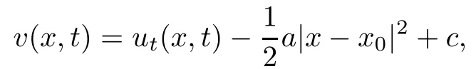
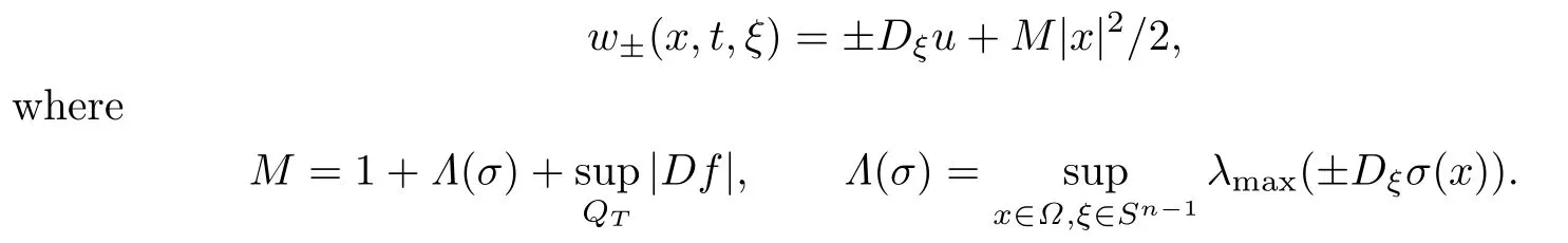
Proof.Choose the function

Therefore,by Lemma 2.2,w+≥u.Similarly,w−≤u.Then there exists a controllable constant C0＞0 such that

This completes the proof.

Theorem 4.2If the assumptions of Theorem1.1hold,then there exists a controllable constantC1＞0such that

holds for all admissible solutionsuof the problem(1.1)–(1.3).

Proof.Step 1.For any ξ∈Sn−1,set

differentiating(1.1)with respect to ξ,we have

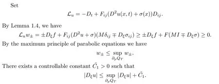
Obviously,Dξu is known onΩ×{t=0}×Sn−1,and hence we only need to get a priori estimate of|Dξu|on∂Ω×[0,T]×Sn−1.

Step 2.For all(x0,t0)∈∂Ω×[0,T],by(1.2)and Theorem 4.1,there exists a controllable constant＞0 such that

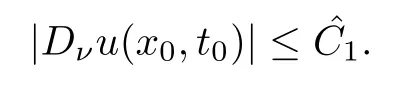
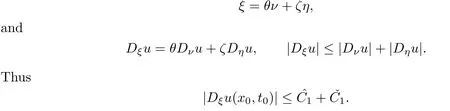
If we can prove that there exists a controllable constant＞0 such that

where ν·η=0,then for any ξ∈Sn−1,there exist θ,ζ∈[0,1]with θ2+ζ2=1 such that

Step 3.We now prove that(∗)holds.Actually,if u(x,t0)is a convex function of x, following the proof of Theorem 2.2 in[8],we have

If it were not true,we could choose the function

Theorem 4.3If the assumptions of Theorem1.1hold,then there exists a controllable constantC2＞0such that

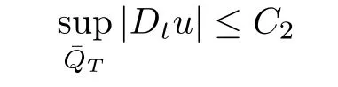
holds for all admissible solutionsuof the problem(1.1)–(1.3).

Proof.A priori estimate

in Theorem 3.1 yields

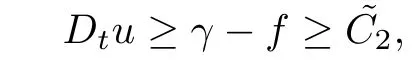
In order to get the upper bound of Dtu,denoting v=Dtu,differentiating(1.1)–(1.2) with respect to t,we have

Following the proof of Theorem 4.1 we get the upper bound of Dtu.Thus the proof of Theorem 4.3 is completed.

By Theorems 3.1 and 4.3,we have the following proposition.

Proposition 4.1If the assumptions of Theorem1.1hold,then there exists a controllable constant Γ＞0such that

for all admissible solutionsuof the problem(1.1)–(1.3).

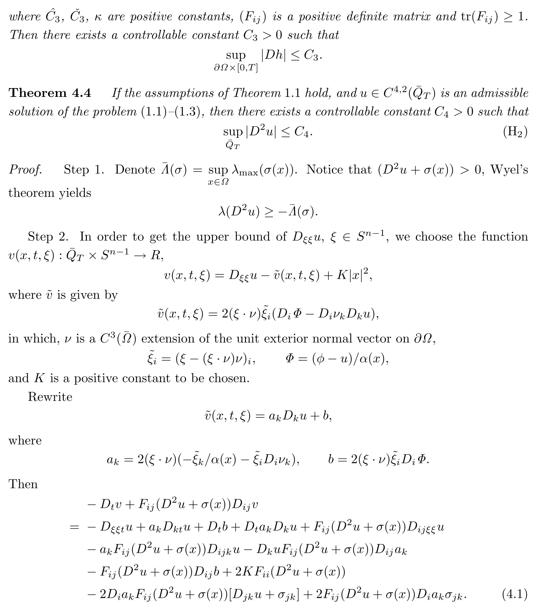
Step 3.From now on,we prove that we can choose K＞0 large enough so that the right hand term of(4.1)is positive.

By Lemma 1.2,we have

differentiating(1.1)twice with respect to ξ∈Sn−1,we get

Since F is concave,it holds that

differentiating(1.1)with respect to xk,and multiplying by ak,we get

Since(Fij(D2u+σ(x)))is a positive de finite matrix,we have

At last,by Lemma 1.3,we have

Substituting(4.2)–(4.5)into(4.1),and noticing that the other terms in the right hand side of(4.1)are all controllable,for all(x,t)∈we have

where C is a controllable constant,and K is a large enough controllable positive constant. By means of the maximum principle of parabolic equations,we know that the maximum of v is attained on∂pQT.

Step 4.Since v is known onΩ×{t=0}×Sn−1,we only need to estimate v on∂Ω×(0,T]×Sn−1.Assume that the maximum of v is attained at(x0,t0,ξ).Then we need only to estimate v(x0,t0,ξ).

Now,we complete the estimate in the following four cases.

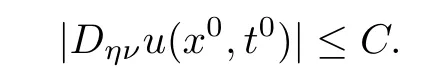
Case 1.Estimate of|Dηνu(x0,t0)|,where ν·η=0.

Set

Applying δito(1.2)(Dνu=Φ),we have

and multiplying(4.6)with ηi,we get

Since ηiνi=0,we have

It holds that

which implies that there exists a controllable positive constant C such that

Case 2.Estimate of|Dηηu(x0,t0)|,where ν·η=0.

Applying δitwice to(1.2)(Dνu=Φ),we have

and multiplying(4.7)with ξiξj,we get

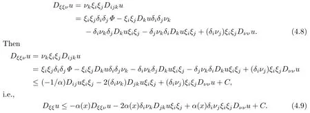
Since the maximum of v is attained at(x0,t0,ξ)∈∂Ω×[0,T]×Sn−1and ak=0(by ξ·ν=0),we have

where C is a controllable positive constant.Moreover,by the positive de finite property of (δiνk)and(Djku+σjk(x)),we have

which implies that

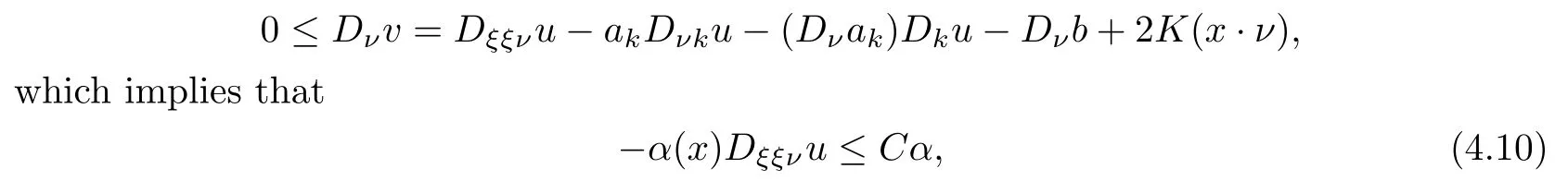
Case 4.Estimate of|Dννu(x0,t0)|.

differentiating(1.1)with respect to xk,we get

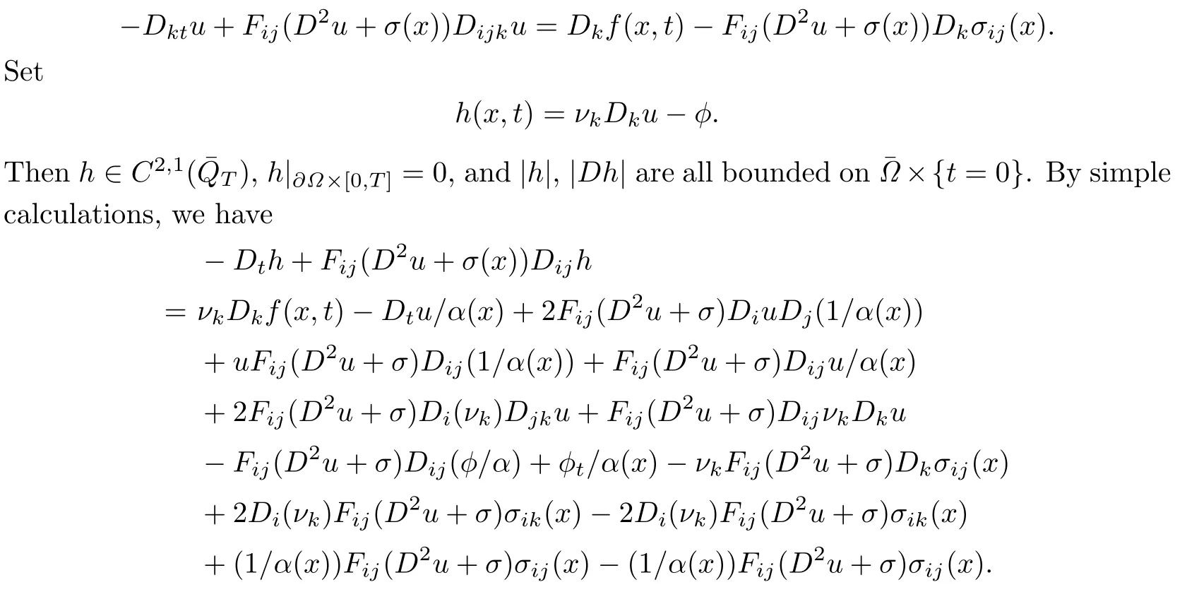
Following the discussion of(4.1),we can find a controllable constant κ＞0 such that

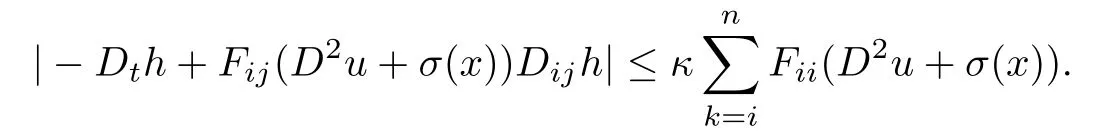
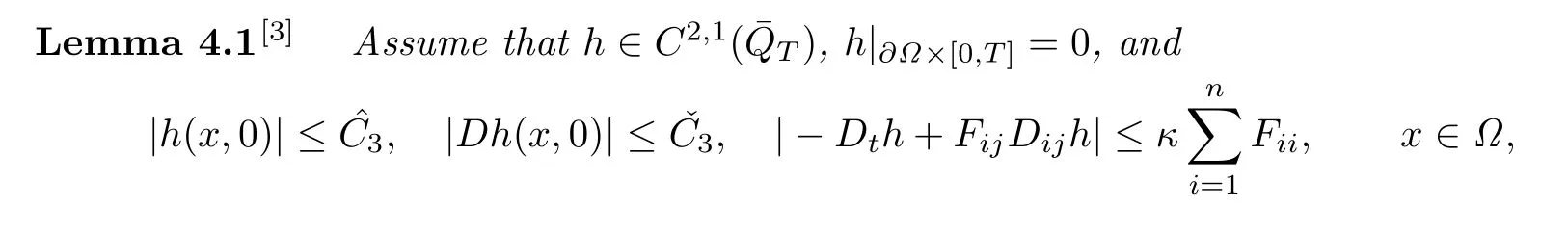
By Lemma 4.1,there exists a controllable constant C3＞0 such that

The proof is completed.

Proof.Let 0＜λ1≤···≤λnbe the eigenvalues of(D2u+σ(x)).Noticing that Dtu and f are bounded,we can find that

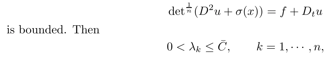
Diagonalizing Fij(D2u+σ(x)),by Lemma 1.2,we see that the eigenvalues of(Fij(D2u+σ(x)) are

AcknowledgmentThe first author is greatly indebted to his thesis adviser Professor Wang Guang-lie and Dr.Ren Chang-yu.

[1]Ca ff arelli L,Nirenberg L,Spruck J.The Dirichlet problem for nonlinear second-order elliptic equations I.Monge-Ampree equation.Comm.Pure Appl.Math.,1984,37:369–402.

[2]Ivochkina N M,Ladyzhenskaya O A.On parabolic equations generated by symmetric functions of the principal curvatures of the evolving surface or of the eigenvalues of the Hessian,Part I: Monge-Ampre equations.St.Petersburg Math.J.,1995,6:575–594.

[3]Zhou W S,Lian S Z.The third initial-boundary value problem for the equation of parabolic Monge-Ampre type.Acta Sci.Natur.Univ.Jilin,2001,(1):23–30.

[4]Ren C Y.The first initial boundary value problem for fully nonlinear parabollic equations generated by functions of the eigenvalues of the Hessian.J.Math.Anal.Appl.,2008,339: 1362–1373.

[5]Horn R A,Johnson C R.Matrix Analysis.Cambridge:Cambridge Univ.Press,1985.

[6]Gilbarg D,Trudinger N S.Elliptic Partial differential Equations of Second Order.2nd ed.New York-Berlin:Springer-Verlag,1983.

[7]Ladyzhenskaya O A,Solonnikov V A,Ural′ceva N N.Linear and Quisilinear Equations of Parabolic Type.Providence,RI:Amer.Math.Soc.,1968.

[8]Lions P L,Trudinger N S,Urbas J I E.The Neumann problem for equations of Monge-Ampre type.Comm.Pure Appl.Math.,1986,39:539–563.

[9]Lieberman G M.Second Order Parabolic differential Equations.Singapore:World Scienti fi c Publ.,1996.

Communicated by Shi Shao-yun

35K55,35A05

A

1674-5647(2012)01-0075-16

date:April 19,2010.

The NSF(10401009)of China and NCET(060275)of China.