3-D VARIABLE PARAMETER NUMERICAL MODEL FOR EVALUATION OF THE PLANNED EXPLOITABLE GROUNDWATER RESOURCE IN REGIONAL UNCONSOLIDATED SEDIMENTS*

LUO Zu-jiang, WANG Yan

School of Earth Sciences and Engineering, Hohai University, 210098 Nanjing, China, E-mail: luozujiang@sina.com

(Received March 15, 2012, Revised July 25, 2012)

3-D VARIABLE PARAMETER NUMERICAL MODEL FOR EVALUATION OF THE PLANNED EXPLOITABLE GROUNDWATER RESOURCE IN REGIONAL UNCONSOLIDATED SEDIMENTS*

LUO Zu-jiang, WANG Yan

School of Earth Sciences and Engineering, Hohai University, 210098 Nanjing, China, E-mail: luozujiang@sina.com

(Received March 15, 2012, Revised July 25, 2012)

Іn order to correctly evaluate the exploitable groundwater resource in regional complex, thick Quaternary unconsolidated sediments, the whole Quaternary unconsolidated sediments are considered as a unified hydrogeological unit and a 3-D unsteady groundwater flow numerical model is adopted. Meanwhile, with the consideration of the dynamic changes of the porosity, the hydraulic conductivity and the specific storage with the groundwater level dropping during the exploitation process, an improved composite element seepage matrix adjustment method is applied to solve the unsteady flow problem of free surface. Іn order to evaluate the exploitable groundwater resource in Cangzhou, Hebei Province, the hydrogeological conceptual model of Cangzhou is generalized to establish, a 3-D variable parameter numerical model of Cangzhou. Based on the prediction of the present groundwater exploitation, and by adjusting the groundwater exploitation layout, the exploitable groundwater resource is predicted. The model enjoys features like good convergence , good stability and high precision.

exploitable quantity of groundwater resource, variable parameters, free surface, 3-D numerical model

Introduction

Іn North China Plain, Yangtze River Delta and North Jiangsu Plain of China, there are huge thick Quaternary unconsolidated sediments, in which several thick porous aquifers are distributed, from top to bottom, which are, respectively, the Holocene phreatic aquifer, the late Pleistocene aquifer, the middle Pleistocene aquifer and the early Pleistocene confined aquifer. They are separated by clayey layers without much water and with very close hydraulic connections between them. Іn groundwater resource evaluations in unconsolidated sediment areas, 2-D models or quasi 3-D models were often used to assess the groundwater resource layer by layer, leading to some results being repeated and some results missing[1,2]. With a real 3-D model, the clayey aquitard among the aquifers are treated as an independent layer to be calculated together with aquifers[3-5], and the deficiency of 2-D andquasi 3-D models with the clayey aquitard being conceptually treated as a leakage can be avoided, thus the accuracy of the results can be greatly improved.

The Quaternary sediments are unconsolidated. With the groundwater exploitation and the water level dropping continuously, the pore water pressure decreases and the effective stress in the soil increases gradually, which makes the soil skeleton compacting, reducing the distance between soil particles and the porosity of aquifer, therefore, the aquifer permeability and the storage ability are reduced gradually[6-8]. Іn groundwater resource evaluation numerical models, the hydraulic conductivity and the specific storage in the seepage equation were often regarded as constants, ignoring the fact that the transmitting and storage ability of an aquifer is decreasing due to the soil skeleton compacting[9,10]. All these lead to the estimation of the exploitable groundwater resources on the higher side. Therefore, the evaluation of the exploitable groundwater resources of unconsolidated sediments with variable parameter numerical models becomes a hot topic for hydrogeologists.

As a 3-D unsteady groundwater numerical model contains a free surface, the successful treatment of thefree surface is directly related to the convergence and the stability of the model[11], and it is also a key element that has to do with its practical applications. Іn this paper, an improved composite element seepage matrix adjustment method is adopted to deal with the unsteady flow problem with a free surface, to overcome the jumping problem of the integral value near the Gauss points, and to solve the unsteady flow problem involved.

This paper studies the groundwater resource evaluation in Cangzhou, Hebei Province, by generalizing the hydrogeological conceptual model of Cangzhou, to establish a 3-D variable parameter numerical model for calculating the exploitable groundwater resource. Based on the prediction of the present groundwater exploitation, and by readjusting the groundwater exploitation layout, the exploitable groundwater resource is evaluated reasonably.

1. 3-D groundwater seepage numerical model

1.1 Governing equation

Based on the continuity principle and the Darcy’s law, with the coordinates in the principal permeability directions of the anisotropic porous media, the 3-D unsteady flow equation for the porous media can be expressed as[12]

where kxx, kyyand kzzare, respectively, the hydraulic conductivity in the principal directions of the anisotropy medium, h is the water head at point (x,y,z) and at the instant t, W is the source and sink terms,ssis the specific storage, t is time, and Ωis the computational domain.

Applying the variational principle, the above boundary value problem can be equivalently expressed in an extreme problem of functional ()Ih, which requires the partial derivative of the functional equal to zero. The 3-D regions are discretized with hexahedrons of 8 nodes, and the implicit difference scheme is adopted to establish the finite element equation. The overall finite element governing equation can be expressed as

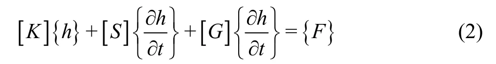
where ｛h｝ is the tested water head vector of the nodes, ［K］ is the overall seepage matrix, which is composed of unit seepage matrix ［K］e, ［S］ is the storage matrix, which is composed of unit specific storage matrix ［S］e, ［G］ is the recharge rate matrix, which is composed by unit recharge rate matrix ［G］e,｛F｝ is the water quantity matrix, which is composed of unit source and sink term matrix ｛E｝eand unit flow boundary matrix ｛｝eQ.

Supposing that ［A］=［K］+(Δt)-1（［S］+［G］）and ｛B｝=｛F｝+(Δt)-1（［S］+［G］）｛h｝, Eq.(2) can be expressed as

where ［A］ is called the global stiffness matrix, and｛B｝ is called the constant term matrix.

1.2 Definite conditions

The initial and boundary conditions for the unsteady seepage calculation are as follows:

(1) Іnitial condition

wher e h0(x,y,z,t0) isthe initialwaterhead at the point (x,y,z).

(2) Boundary conditions

(a) The first kind of boundarycondition

where h1（x,y,z,t） is the known head at the boundary and Γ1is the first kind of the boundary.

(b) The second kind of boundary condition

where q(x,y,z,t)is the recharge capa cityper unit area for the second kind of boundary conditions, cos(n,x), cos(n,y) and cos(n,z) are the directional cosines for th enormal on the body surface and Γ2is the second kind of boundary.

(c) Free surface boundary condition

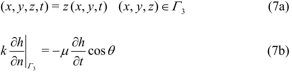
whe re z(x,y,t) is the elevation of free surface,μ is the saturation deficiency (the free surface rise) or the specific yield (the free surface drop),θ is the angle between normal vector of outer boundary and perpendicular direction and Γ3is the free surface boundary.

2. Treatment of free surface and parameters in the model

2.1 Free surface

By decomposing the integral region into triangles, andadopting the high precision numerical integration scheme of the free surface boundary integral term, an improved composite element seepage matrix adjustment method is developed to deal with the unsteady seepage containing a free surface[13].

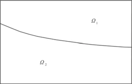
Fig.1 Schematic diagram of real region and imaginary region

Іn the groundwater seepage calculation, the entire computational domain Ω is divided into an imaginary region Ω1and the real region Ω2separated by the free surface (as shown in Fig.1), with its location to be determined in the calculation.

The basic ideas of the improved composite element seepage matrix adjustment method are as follows. By judging the position relation of the free surface and the elements, the elements are identified as real elements, imaginary elements or transition elements. For a node, when h-z＜0 (where h is the water head of the node, z isthe elevation of the node), the node is in the imaginary seepage region and to be classified as an imaginary node. When h-z＞0, the node is in the real seepage region and tobe classified as a real node. When h-z=0, the node is at the free surface. For an element, if its nodes are all imaginary nodes, it will be identified as an imaginary element, while if the nodes are all real nodes, it will be identified as a real element, and otherwise, it will be identified as a transition element. Because there is no seepage in the imaginary element, in the following iterative calculation, to facilitate the calculation, the hydraulic conductivity of the element above the free surface will be multiplied by 1/1 000. For the transition element, according to the equivalent recharge rate to adjust the hydraulic conductivity of the real seepage region, an improved continuous fold line penalty function is used to extend the computational region to the entire element, then the free surface boundary is to be determined iteratively.

The expression ofthe continuous fold line penalty function is chosen as

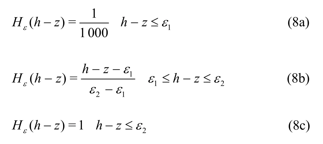
where h is the water head of the node, z is the elevation of the node, ε1takes a negative value and is the maximum verticalprojection of the distance from Gauss point 3 to the free surface when the free surface exactly passes node Ⅲ, ε2is the vertical projection of the distance from Gauss point 1 to the free surface when the free surface exactly passes node Ⅰ (as shown in Fig.2).

Fig.2 Schematic diagram of penalty function parameters

So the seepage matrix for a transition element is

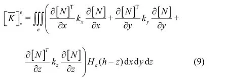
With the use of the continuous fold line penaltyfunct ion, there will be no jumping of the integral value near the Gauss points, and the iteration becomes more stable and easier to converge.

2.2 Parameter dynamic model

2.2.1 Porosity

Theoretically, the dynamic calculation formula of the porosity can be deduced as follows. According to fluid mechanics, the continuity equation of the porous media skeleton is[14]

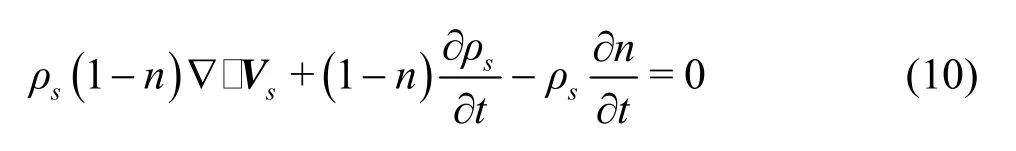
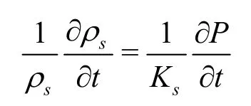
where ρsis the skeleton density, andVsis the velocityof the skeleton particle.

We will have

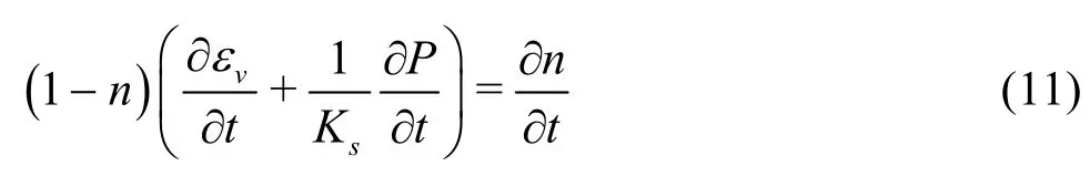
where εvis the volume strain,P is the pore water pressure, Ksis the bulk modulusof elasticity of the porous media skeleton particle, and

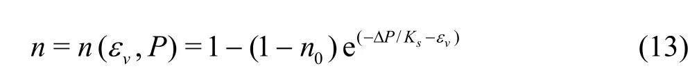
Equation (11) can be integrated to obtain

Іf εv=0, Ks→+∞, then n≡n0. Substituting it into the above equation, we haveC=1-n0, so

Expand ninto Taylor series,

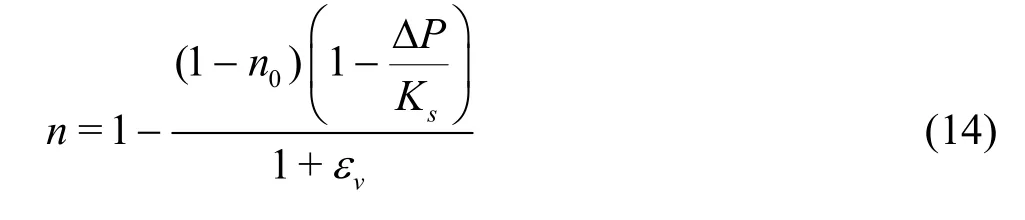
However, the parameters in Eq.(14) are difficult to b e determined. So in the actual application, the dynamic calculation of the porosity can be approximately carried out as follows.

According to 1-D Terzaghi effective stress principle, the vertical deformation of the soil caused by the head changes can be expressed as Δb=-ΔhSskb0, where Δh is the head variation value, b0is the initial thicknes s of the soil and Sskis the skeleton storage of the soil. Supposing that theinitial porosity thickness is b0i, and the vertical deformation caused by the drawdown is Δbi, without considering the lateral deformation, thenthe porosity dynamic change during theexploitation process can be expressed as the primary porosity minus the variation porosity caused by the vertical deformation, as

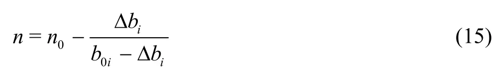
As compa red to the thickness of the soil, the vertical deformation is very small and can be calculated approximately as b0i-Δbib0i. So we have

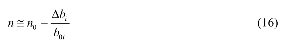
Equation (16) can be usedto calculate the porosity dynamic change.

2.2.2 Hydraulic conductivity

According to the Kozeny-Carman equation, the permeability of an aquifer can be obtained by the following formula[15]

where Spis the surface areaof particles,Sp=As/ Vp, Asis the total area of particles, Vpisthe pore volume, and kzis the Kozney constant.

Let the change of the rock and soi l volume be ΔVb, the change of the particle volume during the seepage process be ΔVr, and the change of the particle area be ΔAs. Іt is assumed that they are all caused by the temperature change,ΔAsis expressed with a coefficient β as

And the cha nges of th e particl e size is expressed as

Then, the change of the porous volume is the difference between the change of the total soil volume and that of the particle size

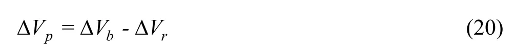
So the new p orosity is

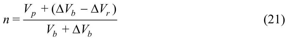
And the new surface area is

From Eqs.(17), (18), (21) and (22) we have

（四）有利于加快农业产业结构调整 标准化、规模化生猪生产的发展，将把畜种、土地等优势资源合理向有能力的人集中，使一部分人从经营者、生产者的双重角色向单一的劳动者转变，改变小而全的生产经营模式，实现产业结构的加速调整和生产的专业化，实现从业人员精力和时间的集中，提高劳动力效率。

From Eqs.(19), (20) and the relationΔVb=εvVb, we have

Substituting it into Eq.(24), we have

Іgnoring the changes in the soil particle surface area and the particle volume during the process of the thermal expansion, the relation among the permeability, the volumetric strain and the initial porosity is as follows

When the change inthe particle volume during the process of the thermal expansion is ignored, according to both Eq.(21) and the relation ΔVb=εvVb, we obtain εv=(n-n0)/(1-n), then the relationship between the permeability and the porosity can be obtained and substituting it intoEq.(27), we obtain

As a result, the relationship between the hydraulic conductivity and the porosity is

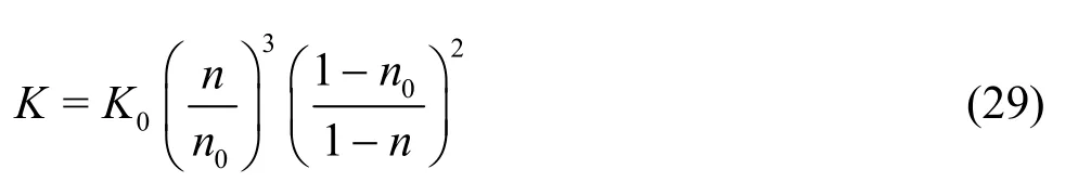
So Eq.(29) can be used to calculate the dynamic change of the hydraulic conductivity.

The dynamic changes of the specific storage can be calculated from thedynamic changes of the porosity.According to the groundwater seepage basic differential equation, the specific storage ssis defined as

whereγwis thewater severity, α is the coefficient of the soilvolume compressibility, and βwis the coefficient of the water volume compressibility.

To sum up, in each calculation step, theporosity is calculated by Eq.(16), then a new value of the hydr aulic conductivity specific storage is obtained by Eq.(29) and Eq.(30), and all new values are substituted into the next step for the parameter dynamic calculation.

3. Solution and finite element method

By using the variational method to discrete the equations, to transform the differential equations into finiteelement equations, and to obtain the initial water head, the boundary conditions, the hydrogeological parameters, the recharge rate and other data, the global stiffness matrix and the constant term are formed. The Preconditioned Conjugate Gradient (PCG) method is chosen for the iterative solution of the finite element equations (Eq.(3)). Іts procedures are as follows. The coefficient matrix of a symmetric positive definite kind is pretreated in order to reduce the condition number of the equivalence, and then the conjugate gradient method is used to enhance the convergence rate and to overcome the numerical instability[16]. A finite element program is developed in Fortran 95language to carry out the 3-D variable parameter numerical simulation of the groundwater. The computing process is described as in Fig.3.

Fig.3 The flow chart of the program

4 . Applications

4.1 Study area

Cangzhou is located at the southeast of Hebei Province. Witha rapid economic development, the water resource is increasingly in demand. Due to the surface water scarcity and the rare average annual precipitation, 85% of the total water consumption comes from the groundwater. The perennial overdraft from the deep groundwater and the exploitation of the mineral water, the geothermal water, the oil and gas and other resources lead to a rapid expansion of the groundwater cone of depression and the serious landsubsidence, which make Cangzhou become a city with the fastest subsiding rate and the biggest subsiding area in North China. Іn order to deal with these environmental problems, a reasonable, optimal exploitation scheme should be established.

4.2 Hydrogeology conceptual model

Consider the unconsolidated Quaternary sediment area of Cangzhou. The main groundwater type is porewater in unconsolidated rock. From high to low, there are the Holocene first aquifer, the late Pleistocene second aquifer, the middle Pleistocene third aquifer and the early Pleistocene fourth aquifer, which all are assumed to be heterogeneous and anisotropic.

The Bohai Sea is taken as the east boundary of the mode l, and the administrative boundary is used as the model boundary in the other three directions. The top boundary is the free surface of the phreatic aquifer, while the bottom boundary is the floor elevation of the fourth aquifer. There is a strong vertical hydraulic connection between aquifers. According to the survey data and the hydrogeology observation data during many years, the top boundary is a recharge boundary, which is recharged by the precipitation and the agricultural irrigation infiltration, and on the other hand, it is also a discharge boundary of the evaporation, so it is assumed to be a free surface boundary, while the bottom boundary is an impermeable boundary, the lateral boundary is assumed to be the general head boundary.

Due to the overexploitation of the third confined aquifer, a large area regional groundwater cone of depression is formed, the vertical hydraulic connection between aquifers is close and complex, and the water head of each aquifer is directly influenced by the groundwater exploitation, so the groundwater flow state is assumed to be a 3-D transient flow.

Fig.4 The mesh of study area

4.3 Mathematical model

The model is 197 500 m × 179 000 m on the plane, while the depthin the vertical direction is 350m. According to the actual hydrogeological structure and geometry, the study area is subdivided into 150×150 rectangular grid cells on the plane, while in the vertical direction it is subdivided into four independent layers, which is the first, second, third, fourth aquifers in the calculation, The total number of effective units is 35 792, and the total effective node number is 46 430. 3-D subdivision grids are shown inFig.4.

The initial flow fields of all aquifers on December 31, 2005 are used as the initial head. Beca use there are not the initial head data for the second and the fourth aquifers, they are obtained by interpolations of the water heads in the adjacent aquifers. The recharge rates of the precipitation and the agricultural irrigation and the discharge rate of the evaporation are treated as the precipitation infiltration rate, and the manual extraction rate is treated as the withdrawal of the pumping well, which is assumed to be an ideal large well. The initial heads of the boundary are given by the initial flow fields for all aquifers. The available information is used as the initial values of each layer parameters. The period from December 31, 2005 to December 31, 2006 is taken as the calibration and verification period of the model, every month is taken as a stress period of the groundwater exploration, and there are 12 stress periods, each of which lasts one time step.

4.4 Calibration and validation

There are a certain number of groundwater level observation wells in each aquifer to fit the groundwater level. The distribution of the observation wells is shown in Fig.5.

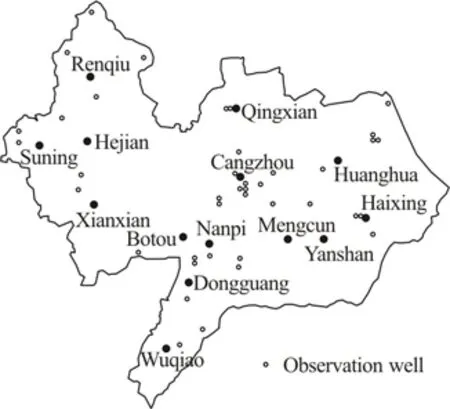
Fig.5 Observation well distribution

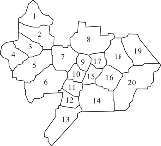
Fig.6 Hydrological parameter zones for aquifer Ⅲ

According to the model calibration and validation processes, the area of all aquifers is divided into 69 parameter zones, and the parameter zones of aquifer Ⅲ are shown in Fig.6 as an example.

Table 1 Initial values of hydrological parameter zones of aquifer Ⅲ

Fig.7 Groundwater level fitting curve on June 30, 2006

Through the calibration and the validation, the initial parameter values of each parameter zone are obtained. Based on these initial values, the groundwater seepage calculation and the parameters dynamiccalculation are carried out. The parameter initial values for each zone of aquifer Ⅲ are shown in Table 1, and the porosity value in each zone of aquifer Ⅲ is given as 0.3 according to related data.

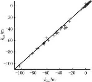
Fig.8 Groundwater level fitting curve on Decembe r 31, 2006

From the results of the calibration, taking the fitting results on June 30, 2006 and December 31, 2006 for examples as shown in Fig.7 and Fig.8, it is shown that the fitting errors of almost all groundwater level observation wells are less than 1m. Іt can be concluded that the parameter values of each zone are all within the water level fitting precision to meet the conventional requirements. According to the calibration process, the general changes of the calculated results agree with those of the observed data, the water exchange strength on boundaries agrees with the actual situation, and the global change trends of the flow field calculated by the model agree with the real cases.

All results reflect well the structure and functional characteristics of the actual groundwater system inthe study area. So the model is credible and canbe used to predict the groundwater system dynamics of Cangzhou.

By analyzing the groundwater system characteristics based on the e xploitation circumstances, combined with the groundwater level constraints of each aquifer, and with the adjustment of the layout of the existing groundwater exploitation, the exploitable quantity of the groundwater is predicted. To adjust the existing groundwater exploitation distribution of Cangzhou, one should follow the following principles:

(1) The lowest groundwater level of every aquifer should not be lower than the top of the aquifer.

(2) The existing layout of the groundwater exploitation should be adjusted to meet the present demands of counties and cities, and to make the largest exploitable resources of the groundwater available with all controllable conditions.

4.5.1 Prediction of groundwater exploitation

With the layout of the groundwater exploitation

4.5 Prediction for planned groundwater exploitation in 2006 of Cangzhou, the groundwater level of the study area is predicted. Simulation results show that the groundwater level of each aquifer drops with years, and the area of the cone of depression expands gradually.

The water level of aquifer І changes less, with the lowest water level changing from -10.1 m on December 31, 2006 to -16.1 m on December 31, 2020. The lowe st water level of aquifer Ⅱ varies from -53.3 m on December 31, 2006 to -66.3 m on December 31, 2020. Aquifer Ⅲ is the main exploitation aquifer, with the biggest groundwater level drop of more than 20 m on December 31, 2020 as compared to the level on December 31, 2003. The lowest water level of the confined aquifer Ⅳ drops from -118.8 m on December 31, 2006 to -140.2 m on December 31, 2020.

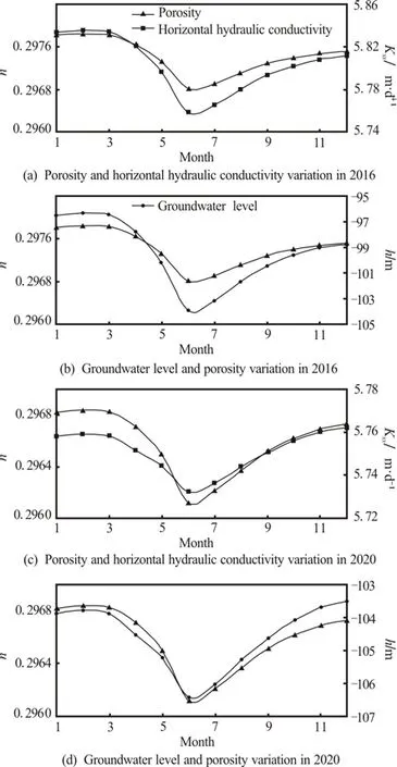
Fig.9 Variation relationship of porosity, groundwater level and horizontal hydraulic conductivity

To prevent the area of the cone of depressionexpanding more seriously, a rational planning should be carried out, and the reasonableness of the exploitationshould be verified.

4.5.2 Prediction for planned groundwater exploitation

Based on the exploitation layout of 2006, the present layout is adjusted to meet the requirement of contr olling the lowest grou ndwater level at the end of 2020.

The analysis mentioned before shows that the parameters change with the groundwater level. Along with the groundwater seepage prediction, the variation values of the parameters can be obtained. Іn Fig.9, the number 9 zone of aquifer Ⅲ that contains the urban area of Cangzhou and the observation well Qing25-4 is taken as an example, to show the variation relationship of the porosity, the groundwater level and the horizontal hydraulic conductivity in 2016 and 2020.

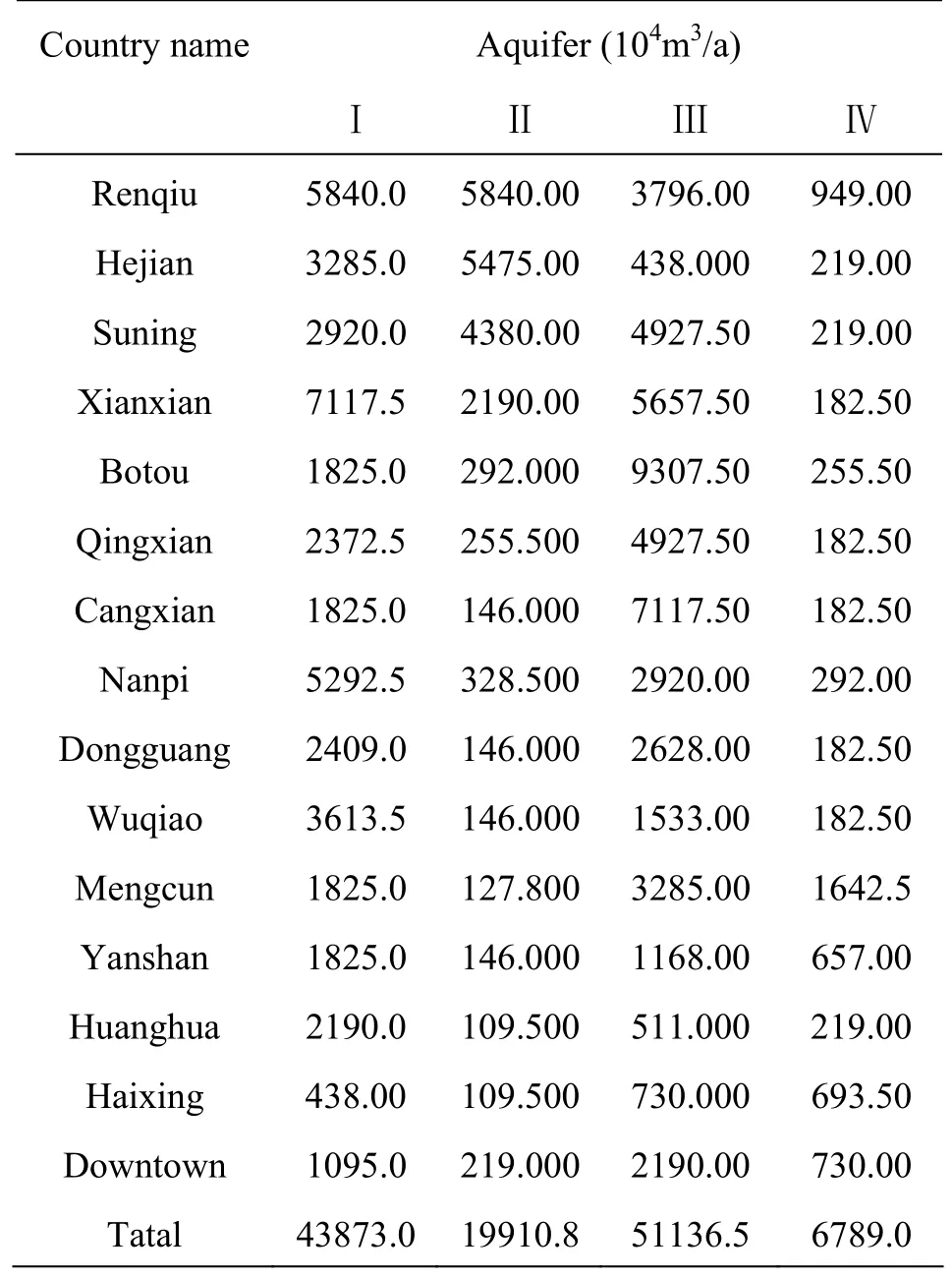
Table 2 Planned exploitable groundwater resource in each country of Cangzhou

With the variable parameter numerical model, the planned exploitable groundwater resource in each country is evaluated as shown in Table 2, and the seepage field of aquifer Ⅲ at the end of 2020 is taken as an example and shown in Fig.10.

Compared with that in 2006, the exploitable groundwater resources in aquifer Ⅰ, aquifer Ⅱ and aquifer Ⅲ increase slightly in the mass, and there is a large increase in aquifer Ⅳ. The exploitable quantity of the groundwater in different regions at the same aquifer is adjusted, being cut down in the center of each groundwater cone of depression, and increased at the regions with a higher groundwater table. As for aquifer Ⅰ and Ⅲ, the quantities at the cone of depressions in Cangzhou, Huanghua, Qingxian, Renqiu, Hejian etc., are cut down and for aquifer Ⅱ and Ⅳ, they are increased at the regions of less extraction areas or no extraction areas.

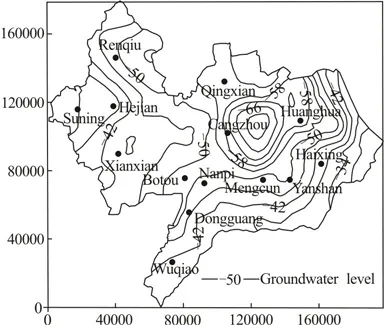
Fig.10 Prediction of planned seepage field of aquiferⅢ on December 31, 2020 (m)

From the prediction for planned cases, it can be seen that the trends in the expansion of the coneof depressions in all aquifers tend to be flattened after 2018, and the groundwater level becomes stable after 2020 , the groundwater level is higher than the top of aquifers, which meets the requirements for the groundwater level control.

5. Conclusions

(1) With the 3-D groundwater seepage numerical model, the complex and thick aquifer system of the regional unconsolidated sediments is evaluated as a unified geological unit, with the aquitard being regarded as a single layer to be calculated together with aquifers, avoiding the repeated calculations when the hydraulic connection between aquifers is treated as a leakage item as in a usual approach, improving the accuracy of the calculation.

(2) Considering the dynamic changes of the porosity, the permeability coefficient and the specific storage with the dropping of the groundwater level and the compacting of the aquifer, the hydrogeologyical unit structure in Quaternary unconsolidated sediments is made more realistic, which greatly improves the confidence level of the calculation.

(3) The application of the improved composite element seepage matrix adjustment method successfully overcomes the jumping of the integral quantity near Gauss points, and it can effectively be used tosolve the problem of the 3-D unsteady flow of the groundwater with free surface.

(4) The evaluation of the planned exploitable quantity of the groundwater can avoid the sharp dropping of the groundwater level, the land subsidence and other geological environment problems caused by the mass exploitation of the groundwater at a local area, to achieve the sustainabledevelopment and utilization of groundwater resources.

[1] YE Shu-jun, DAІ Shui-han. Comparing of results of two dimensional, quasi three dimensional and three dimensional models for groundwater[J]. Hydrogeology and Engineering Geology, 2003, 30(5): 23-27(in Chinese).

[2] XUE Yu-qun. Present status of modeling land subsidence in China and problems to be solved[J]. Hydrogeology and Engineering Geology, 2003, 30(5): 1-5(in Chinese).

[3]EBRAHEEM A. M., GARAMOON H. K. and RІAD S. et al. Numerical modeling of groundwater resource management options in the East Oweinat area, SW Egypt[J]. Environmental Geology, 2003, 44(4): 433- 447.

[4] NASTEV M., RІVERA A. and LEFEBVRE R. et al. Numerical simulation of groundwater flow in regional rock aquifers, south-western Quebec, Canada[J]. Hydrogeology Journal, 2005,13(5-6): 835-848.

[5]BAUER P., GUMBRІCHT T. and KІNZELBACH W. A regional coupled surface water/groundwater model of the Okavango Delta, Botswana[J]. Water Resources Research, 2006, 42(4): 1435-1449.

[6]TAN Guang-ming, JІANG Lei and SHU Cai-wen et al. Experimental study of scour rate in consolidated cohesive sediment[J]. Journal of Hydrodynamics,2010, 22(1): 51-57.

[7]WU Ji-chun, SHІ Xiao-qing and YE Shu-jun et al. Numerical simulation of land subsidence induced by groundwater overexploitation in Su-Xi-Chang area, China[J]. Environmental Geology, 2009, 57(6): 1409-1421.

[8] ZHANG Yun, XUE Yu-qun and Wu Ji-chun et al. Excessive groundwater withdrawal and resultant land subsidence in the Su-Xi-Chang area, China[J]. Enviro- nmental Earth Sciences, 2010, 61(6): 1135-1143.

[9] SHІ Liang-gong, CAІ Li and SHІ Lun-yang. The microscopic characteristics of Shanghai soft clay and its effect on soil body deformation and land subsidence[J]. Environmental Geology, 2009, 56(6): 1051-1056.

[10]GLOWACKA E., SARYCHІKHІNA O. and NAVA F. A. Subsidence and stress change in the Cerro Prieto Geothermal Field, B. C., Mexico[J]. Pure and Environmental Science, 2005, 162(11): 2095-2110.

[11]MJІEMAH І. C., CAMP M. V. and MARTENS K. et al. Groundwater exploitation and recharge rate estimation of a quaternary sand aquifer in Dar-es-Salaam area, Tanzania[J]. Environmental Earth Sciences, 2011, 63(3): 559-569.

[12]WU Ji-chun, XUE Yu-qun. Groundwater dynamics[M]. Beijing: China Water Power Press, 2009(in Chinese).

[13]LUO Zu-jiang, LІ Hui-zhong and FU Yan-ling. Three dimensional numerical simulation of groundwater dewatering and land-subsidence control in quaternary unconsolidated sediments[M]. Beijing: Science Press, 2009(in Chinese).

[14]ZHANG Kai, ZHOU Hui and FENG Xia-ting et al. Discussion onforms of continuum equation for Biot’s consolidation[J]. Rock and Soil Mechanics, 2009, 30(11): 3273-3277(in Chinese).

[15]MAVKO G., MUKERJІ T. and DVORKІN J. The rock physics handbook: Tools for seismic analysis in porous media[M]. Cambridge, UK: Cambridge University Press, 2003.

[16]LUO Zu-jiang, ZHANG Ying-ying and WU Yong-xia. Finite element numerical simulation of three-dimensional seepage controlfor deep foundation pit dewatering [J]. Journal of Hydrodynamics, 2008, 20(5): 596-602.

DOІ: 10.1016/S1001-6058(11)60324-7

* Project supported by the Major Research Project of Hebei Province (Grant No. CZCG2008008).

Biography: LUO Zu-jiang (1964-), Male, Ph. D., Professor