APPLICATION OF QUADRATIC AND CUBIC TURBULENCE MODELS ON CAVITATING FLOWS AROUND SUBMERGED OBJECTS*
2012-08-22CHENYing
CHEN Ying
Department of Engineering Mechanics, Shanghai Jiao Tong University, Shanghai 200240, China,
E-mail: cyofjs@sjtu.edu.cn
LU Chuan-jing
Department of Engineering Mechanics and State Key Laboratory of Ocean Engineering, Shanghai Jiao Tong University, Shanghai 200240, China
CAO Jia-yi, CHEN Xin
Department of Engineering Mechanics, Shanghai Jiao Tong University, Shanghai 200240, China
(Received February 26, 2012, Revised June 16, 2012)
APPLICATION OF QUADRATIC AND CUBIC TURBULENCE MODELS ON CAVITATING FLOWS AROUND SUBMERGED OBJECTS*
CHEN Ying
Department of Engineering Mechanics, Shanghai Jiao Tong University, Shanghai 200240, China,
E-mail: cyofjs@sjtu.edu.cn
LU Chuan-jing
Department of Engineering Mechanics and State Key Laboratory of Ocean Engineering, Shanghai Jiao Tong University, Shanghai 200240, China
CAO Jia-yi, CHEN Xin
Department of Engineering Mechanics, Shanghai Jiao Tong University, Shanghai 200240, China
(Received February 26, 2012, Revised June 16, 2012)
Quadratic and cubic Non-Linear Eddy-Viscosity Models (NLEVMs) at low Reynolds number (Re) correction were introduced into the present Computational Fluid Dynamics (CFD) framework, to provide better numerical treatment about the anisotropic turbulence stress in cavitating flows, which have large density ratio and large-scaled swirling flow structures. The applications of these NLEVMs were carried out through a self-developed cavitation code, coupled with a cavitation model based on the transport equation of liquid phase. These NLEVMs were firstly validated by the benchmark of disk supercavity, and found able to obtain more accurate capture of the hydrodynamic properties than the linear models. One of such models was further applied on the cavitation problem of submerged vehicles. Ultimately, the supercavitating flows around an especially designed underwater vehicle were predicted using the cubick-ε turbulence model, and its cavitation behaviors were studied.
cavitating flow, Non-Linear Eddy-Viscosity Model (NLEVM), submerged object, cavitation model
Introduction
As a fundamental property of liquid, cavitation often occurs in a wide range of industry flows, and usually causes some undesirable characters like cavitation erosion, noise and vibration. However, supercavitation has been utilized as a perspective method for the drag reduction of high-speed underwater vehicles. Savchenko[1]conducted experimental studies on the supercavitating flows around disk cavitators, and concluded an empirical formula for the cavity profile. Vlasenko[2]experimentally investigated the hydrodynamics of the axisymmetric body moving in supercavity, and qualitatively described the shapes of the cavities.
As for the numerical simulation of cavitatingflows, CFD framework based on the solving of the Reynolds Averaged Navier-Stokes (RANS) equations has already been proved its capability. Merkle et al.[3]and Qin et al.[4]suggested the Homogenous Equilibrium Model (HEM) based on the barotropic state equation of the mixture. This approach was also used by Byeong et al.[5]and Goncalves and Patella[6]to predict the periodic internal cavitating flow through a duct. Kunz et al.[7]proposed another HEM based on the transport equation of the phase fraction to simulate partial cavitation. This model was popularly applied by researchers, like Chen et al.[8,9], Hejranfar and Fattah-Hesary[10]and Shams and Apte[11]et al. Subsequently, Yuan et al.[12]and Singhal et al.[13]proposed other such kind of models deduced from the Rayleigh-Plesset bubble dynamics equation. Saito et al.[14]further expressed the saturated vapor pressure as a function of temperature in their model. Owis and Nayfeh[15]proposed a method of employing such model as well as the Peng-Robinson state equation ofliquid and vapor phases to simulate the compressible cavitating flows.
However, those numerical works were primarily coupled with the Linear Eddy-Viscosity Models (LEVMs), in which the isotropic hypothesis between the Reynolds stresses and the rate of strain made the anisotropic stresses omitted. Consequently, the linear models have been known to fail in complex flows. As far as cavitation is concerned, the cavitated region is filled with the mixture of large density ratio and complicated swirling structure. Non-Linear Eddy-Viscosity Model (NLEVM) has aroused significant interests since the last decade because of their potential in obtaining better prediction than linear models. The application of the NLEVM on cavitating flows has seldom been carried out so far.
The primary aim of this work is to examine whether the NLEVM coupled with the present HEM can provide more accurate results in the numerical prediction of cavitating flows. In the present work, computations were carried out using linear and nonlinear models on the benchmark of the cavity around disk which has analytical solution and experimental results. Detailed comparisons between the numerical results of some kinds of NLEVMs were conducted. Through validation these models were extended to the applications in the cavitating flows around the objects with more complicated shapes.
A self-developed computational code was used to simulate the 3-D flows. This code was developed with the Finite Volume Method (FVM) employing an implicit segregated solver, and is applicable to the computational domain divided by body-fitted multi-block structured mesh.
1. Mathematical model
1.1 General governing equations
The mathematical model of the HEM approach consists of the mixture’s continuity equation, the momentum equation, the turbulent kinetic energy balance equation, and the equation controlling phase-transition. In cavitating flows, density is entirely non-uniform in the cavitated region, and the velocity divergence does not disappear automatically. Thus, the complete forms of the governing equations were used as follows:
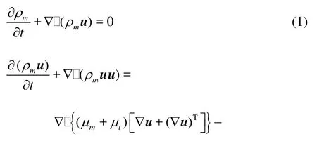

where ρmand μmare respectively the density and the molecular viscosity of the mixture and will be formulated in the following subsection, S denotes the rate of strain tensor,R' in the momentum equation is the additional non-linear Reynolds stress tensor.
1.2 Nonlinear turbulence models
In the current mathematical model, the linear part of the turbulence stress is considered to keep linear relation with the rate of strain as described by the Boussinesq hypothesis. The eddy-viscosity μtis calculated using the turbulent kinetic energy k and the dissipationε. The linear k-ε model with low Recorrection and the local linear realizablek-ω model were adopted to construct the NLVEM used in the present work. The following k equation is identical for each model
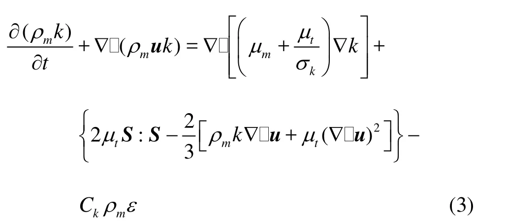
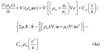
Other governing equations for the kε- model and the kω- model are listed below respectively.
For the low Re linear kε- model
For the local linear realizable kω- model
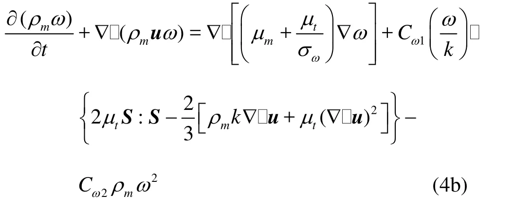
where σk,σεand σωare the Prandtl numbers, Ck, Cε1, Cε2, Cω1and Cω2are model parameters with corrections for lowRe situations, the turbulence viscosity will be reducedas the wall is approached in near-wall flows.
In the present work,the quadratic and the cubic mod els were employed. The additional non-linear parts of the Reynolds stresses were added. The quadratic stress-strain relation was first suggested by Myong and Kasagi. Here, the full form with compressible corrections was employed to consider the inherent compressibility of the cavitating flows.
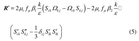
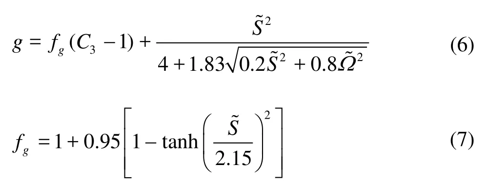
where Si'j=Sij-1/3δijSllis a correction for the rate of straintensor Sij, Ωijis the rate of rotation tensor, fμis the low Re coefficient, β1=g-1(1-0.5C1), β2=g-1(2-C2)a re experimentally obtained coefficients,in which theg is formulated in the following equations:
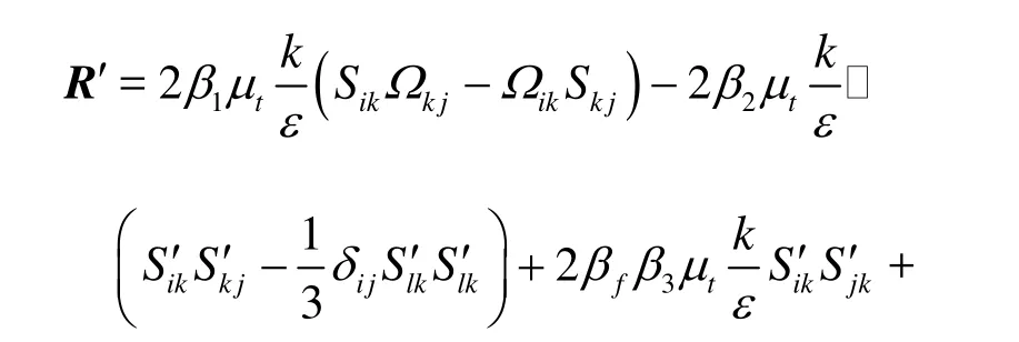
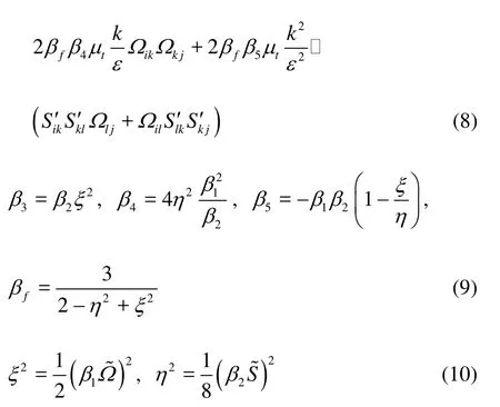
The cubic terms in the stress-strain relation were introduced to acquire a higher order non-linear model. Craft et al. proposed a cubic NLEVM which includes all the possible cubic terms. In the present work, a similar model was adopted. The cubic Reynolds stress is
1.3 Cavitation model
The cavitation model employed in the present work is an improvedversion of that of Kunz etal.[7]. In the present model, the mass fraction equation of the liquid phase was solved. The liquid continuity equation holds as
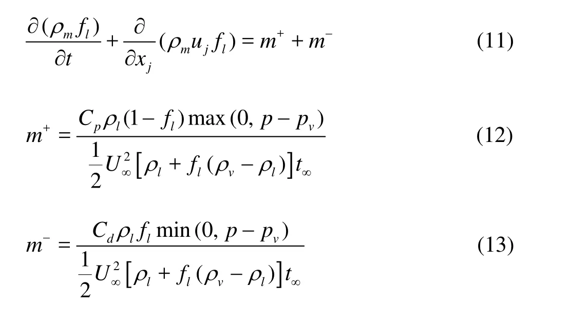
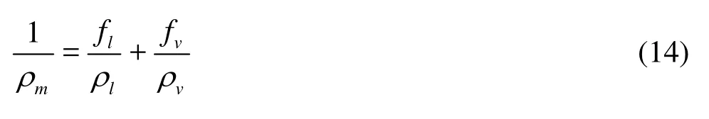
where the subscripts l and vrepresent liquid and vapor respectively,t∞indicates the time scale of the mean flow, U∞is thevelocity of the free-stream,f is mass fraction, and Cpand Cdare empirical constants. This can be referred from the authors’ previous work[7]. The mixture density ρmis formulated as
2. Numerical methodology
The Navier-Stokes equations were solved in a 3-D domain divided by multi-block body-fitted structured mesh. The FVM was used to discretize the gove-rning equations. An implicit segregated solver was constructed to decouple and solve the non-linear equations.
The transient term was approximated with a three time-leve l scheme with second-order accuracy. The conv ective flux was treated as the combination of an implicit first-order upwind scheme and an explicit higher-order scheme with deferred correction, to make a compromise between the convergence, stability, and accuracy. The diffusive flux was also mixed of implicit first-order scheme and deferred correction term of central scheme.
In the numerical aspects of cavitation modeling, the mass fraction equation of liquid phase was handled using the integral form in conjunction with the continuity equation to obtain a discretized algebraic equation with the benefit of diagonally dominant coefficient matrix. The resulted linear equation system for each governing equation at each time step was solved iteratively using the Strongly Implicit Procedure (SIP).
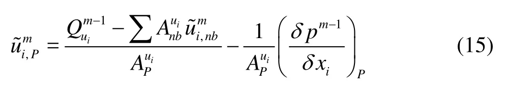
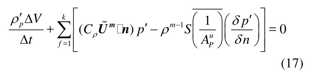
A procedure for pressure-velocity-density coupling correction was carried out to deal with the compressibility character of cavitating flows. After discretizing the momentum equation, two computation steps were executed in each time step. The first step is to solve the linear equation by the iteration cycle. Equation (15) denotes the number-m iteration step, in which the number-m intermediate velocity fieldis calculated using pm-1and U~m-1obtained in the previous step.
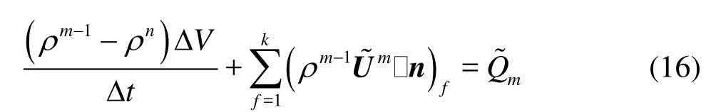
After putting the upper equation together with the discretized continuity equation and the correction relations of ρn+1=ρm-1+ρ', Um=+U' and pm=pm-1+p ', and omitting the higher-order quantities, the total correction equation was rearranged as Eq.(17). The corrections of pressure, velocity and density can be ultimately given using this equation and the compressibility relation betweenρ' and p'.
3. Problem statement and preconditions
In the following sections, the flows around several objects are investigated. These objects are disk cavitator, simple head axis-symmetric body, and a kind of submerged vehicle with complex shape.
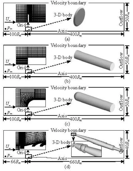
Fig.1 Sketch of 3-D objects and computational domain
In Fig.1, the 3-D shapes of the bodies as well as the configuration of the computational domains are illustrated, where Rndenotes the radius of the disk cavitator or the cylinders, which are 0.01 m. In all the following, the working medium is water at the temperature of 293 K, for which the saturated pressure is about 2 350 Pa and the surface tension is about 0.0717 N/m. The densities of pure liquid and3vapor composing3the mixture are 1 000 kg/m and 0.5542 kg/m respectively. The computations of the cavitating flows were carried out as a full unsteady process. The time step was set to Δt=0.1Rn/U∞.
The cavitation number σ is a primary parameter in cavitating flows. The cavitybody lengthens along with the depressing of cavitation number. The computations in this paper weremainly carried out inthe range of σ<0.1. The combination of the NLEVMs with the present cavitation model gives good convergence property. Figure 2 shows the graphs of a typical convergence history of the momentum equation and the conservation equation.
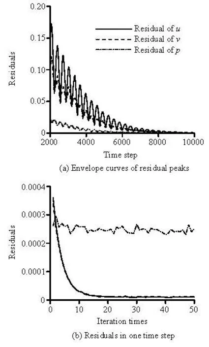
Fig.2 Residual history in the computation process ofsteady cavity
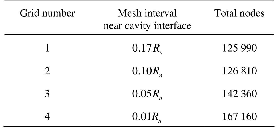
Table 1 Scales of the series of grids
A series of computational meshes with different grid finenesses were tested to choose an appropriate one. The four meshes are listed in Table 1. Firstly, trialcomputations about the disk supercavity were performed on the four grids under the same flowing condition, with a free stream of Re≈105and σ= 0.1.
Since in practical applications the dynamic characters of supercavity are primarilydetermined by its scales, the mesh influences on the cavity interface thick ness ΔR and the cavity radius R are especially concerned. ΔR is defined as the transverse distance across which the mixture density ρmvaries from 0.1ρlto 0.9ρl. The radius R is defined as the transverse distance from the cavity axis to the position where the density is equal to 0.5ρl. Table 2 shows the relative decrement ratio of the computed cavity interface thickness between two neighboring grids. It is apparent that the change rate of ΔR from grid-3 to grid-4 is entirely below 3%, which will be small enough for regarding the grid-3 as adequate to capture the detail of the cavity.
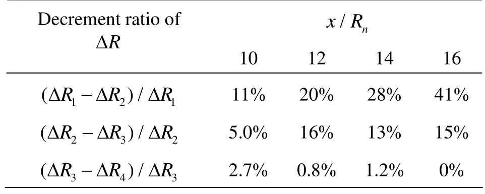
Table 2 Decrement ratio of the cavity interface thickness between two neighboring grids
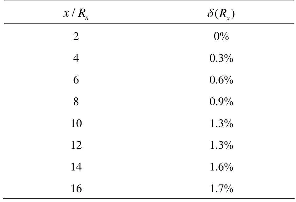
Table 3 Relative standard deviationof the cavity radiuses computedondifferent grids
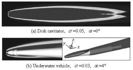
Fig .3 Computed supercavities over objects (in contour and isosurface of vapor fraction)
Table 3 presents the relative standard deviation of the cavity radius R computed on the series of grids. The tiny deviations indicate that little difference exists b etwee n the cav ity radiuse s usin g g rids with distinctmeshfineness,incontrastwiththeconditionof ΔR. This is because the cavity radius is measured at the location of ρm=0.5ρl, and the augment or reduction of ΔR on different grids approximately occurs around the position of abo ut ρm=0.5ρl.
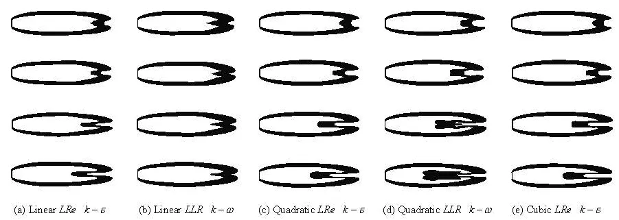
Fig.4Time series of the predicted supercavities over disk cavitator by various turbulence models (σ=0.1)
Fi g.5 Evolution of cavity profile deduced by different turbulence models
The above dependency demonstrated that grid-3 can be used to capture both sufficiently accurate detailed i nformation and macroscopic size for supercavity. Thi s grid will be adopted in the following sections of this paper.
4. Results and discussion
In this section, the quadratic and the cubic NLEVMs co upled with the HEM based numerical methods were firstly verified by benchmark problems,and further utilized to simu late more complicated 3-D cavi tating flows. First of all, the advantage of NLEVM was estimated by comparing its computational results with those of linear models in the aspects of cavity character and hydrodynamics property. Figure 3 presents a preview of the typical supercavity around the disk cavitator and underwater vehicle.
4.1 Verification of NLEVM by the supercavity around disk cavitator
Naturally generated supercavity usually has a large scale of streamline curvature along the cavity interface, and involves a large region of swirling vapor structure inside the cavity. These factors urge the numerical works to meet challenge in keeping the cavity interface stable as in experiments. The main difficulty lies in the accurate description of the viscosity around the interface across which great anisotropy of turbulence stress exists. NLEVM just has the advantage of effectively describing the viscous forces along the cavity interface.
Comparison between the shapes of disk cavities simulated using the NLEVMs and LEVMs are presented in Fig.4, in which each cavity is shown with the density range varying from0.1ρlto 0.9ρl. For the case of each turbulence model, the cavity shapes of four moments with same time interval after the cavity reaches its maximal length are listed. It is obvious to notice that, the cavity interface calculated by the LEVM continues fluctuating along with the development of the re-entrant flow. However, the NLEVM evidently restrains such fluctuation and makes the obtained cavities more stable all the while. This can be explained as a result of the fact that the NLEVM gives a better distribution of the effective viscosity near cavity interface due to the effect of the non-linear Reynolds stresses:
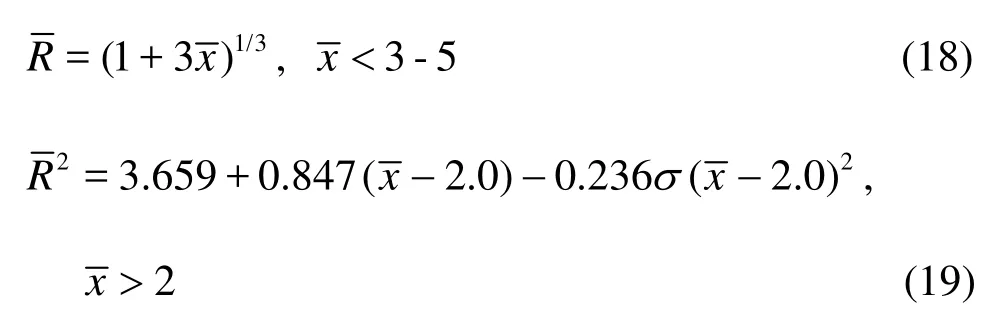
Furthermore, the profiles of the cavities were quantitatively contrasted with the empirical formula which was mathematically fitted from experimental data by Logvi-novich in 1973, as shown in Eqs.(18) and(19). Since the numerical cavity interface always has certain thickness with density transition, the cavity profile of ρm=0.5ρlis selected to compare with the empirical formula, in which,=x/Rnand=R/ Rn.
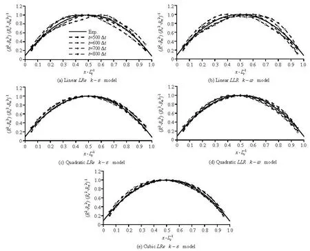
The detailed comparisons are shown in Fig.5, in which each graph corresponds to one turbulence model. The four curves in each graph represent the four moments with same time interval. In the figure, Lcand Rcdenote respectively the maximal length and radius of cavity, and Δt is the time step in the unsteady flow computation.
The comparison indicates that all these turbulence models can obtain cavity profiles approximately around both sides of the profile curve of the experimental empirical formula, as shown by the solid line in the figure. However, the linear models induce strong surface fluctuations around the equilibrium position of average cavity radius, and bring a deviation from experimental result with error of up to 16%. The cavity profile has peak or valley value alternately at the left half and right half of the cavity, or heaves on the middle of cavity. That is to say, the LEVM is hard to obtain stable cavity shape when the cavity grows into supercavity. On the other hand, such fluctuation of cavity interface was effectively eliminated while the NLEVMs were applicable. In this case, the cavity profiles of the different moments congregate closely without vibration and approach the experimental empirical formula with an error of about 5%, which is much more accurate than those by the LEVMs. Meanwhile, there seems to be no evident difference between the results of quadratic model and cubic model. It indicates that quadratic NLEVM is sufficient to describe the anisotropy of the Reynolds stresses in the case of supercavitating flows, at least in combination with the present cavitation model.
4.2 Influence analysis of vehicle shape to the cavity properties
In this subsection, the quadratic non-linear kε model is applied to the cavitating flows around submerged vehicles with simple shape. As one knows, the flow structure around object is crucially influenced by the body’s scale and shape. This is especially important in the case of cavitating flows, where the pressure distribution plays a pivotal role.
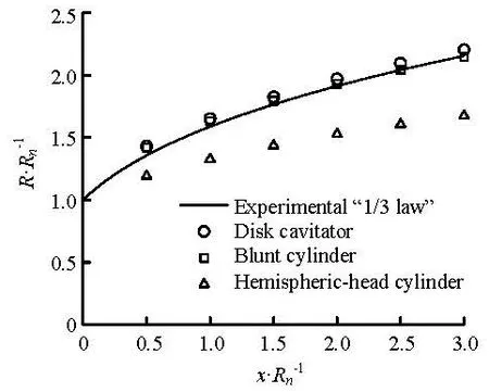
Fig.6 Computed front part of the cavity profiles vs. experimental result (σ=0.1, quadratic low Re modified kε model)
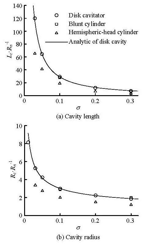
Fig.7 Cavity scales at different cavitation numbers (quadratic low Re modified k-ε model)
Underwater vehicle with smooth head was regarded unable to create cavity of the same size as the vehicle with blunt head. The smooth head of the cylinder causes the cavity size to be markedly reduced fromthat of the disk cavitator. Such effect could be demonstrated by Fig.6, in which the solid line represents the empirical formula of disk cavity profile as Eq.(18) which is called “1/3 law”. In the figure, the front section profiles of the cavities over a blunt cylinder and a hemispheric-head cylinder are compared with that of the cavity over the disk cavitator with same diameter. Little difference is found to exist between the cavity profiles of the disk and the blunt cylinder. Nevertheless, the cavity radius for the hemispheric-head cylinder is markedly smaller than the ones for the former two.
Furthermore, in Fig.7 the calculated cavity length Lcand maximal radiusRcwere compared with the analytical solution of disk cavity given by Garabedian in1956, shown in Eq.(20). The cavity interfaces whereρmequal to 0.8ρland 0.5ρlwere defined as the cavity length and the radius. The cavity dimensionsof the blunt cylinder are close to those of the disk cavitator and approximately accord with the analytical ones. However the cavity sizes of the hemispheric-head cylinder are distinctly smaller than those of the disk and the blunt cylinder. Definite conclusion could be drawn that the head shape of vehicle is a more important factor than the main body in the influence on cavity shape.
Fig.8 Pressure coefficient distribution along thehemisphericheadcylinder surface (quadratic low Re modified kε model)
Figure 8 describes the pressure coefficientdistribution along the cavity encapsulated vehicle’s surface. Inthe figure, s denotes the distance from the front stagnation point of the cylinder along the wall surface, and Dndenotes the vehicle’s diameter. The numerically predicted pressure agrees well with the experiment. The most important fact to be noticed is that some typical characters were captured, such as the invariable vapor pressure inside cavity, the range of cavitating region, and the position and extent of the pressure peak near the cavity closure.
The dynamic character of supercavity is always particularly cared among the entire flow aspects in supercavitating flows, due to its crucial function on the drag reduction effect of supercavity. The numerical methods should effectively reveal the hydrodynamic forces acting on the vehicle body. Table 4 lists the predicted drag coefficient of the disk cavity in contrast with the analytical solution of potential flow expressed as Cd=Cd0(1+σ), in which Cd0=0.82 denotes the drag coefficient as σ approaches zero. Table 4 shows that almost all the values of relative error εCdbetween the numerical and the theoretical results at various cavitation numbers are around 2%. This indicates the prediction accuracy of the numerical method and exhibits a force reduction trend when cavitation number drops. Table 5 further compares the numerically predicted drag coefficients of the three cavity encapsulated objects. According to the validation ofthe prediction of disk cavity shown in Table 4,a similar conclusion about the impact of cavitator shape on the drag force as to the cavity scale can be drawn from Table 5 that, vehicle’s cylinder body has little influence to the drag force if only it has the same blunt head as disk cavitator, while the smooth shape of the hemispheric-head cylinder vehicle makes the drag force depressed much greatly than the blunt ones.
Table 4 Drag coefficient of disk cavity at different cavitation number
Table 5Predicted drag coefficients of the cavity wrapped objects
4.3 Application of cubic NLEVM to the cavitating flow around complex vehicle
Apractical submerged vehicle withmorecomplex shape was designed, as shown in Fig.1. This complex vehicle consists of one disk cavitator and two bowls acting as gas ventilation port and one cylindrical pillar for fastening in practical application. In this subsection, the cubic non-linear k-ε model was utilized to the numerical inve stigation of conformation and hydrodynamics of the cavity around this vehicle.
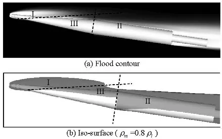
Fig .9 Flood contour and iso-surface (ρm=0.8ρl) ofthe numerically predicted three-segment supercavity using cubic lowRe modified k-ε model (σ=0.03,α=8o)
Figure 9 gives a typical image of the predicted supercavity at a comparatively low cavitation numober of σ=0.03and a large angle of attack ofα=8. In such condition the vehicle is entirely encapsulated by the cavity which is typically composed of three parts. Figure 10 systematically lists the simulated cavity figures near the conical segment of the vehicle in various conditions of cavitation number and angle of attack. The cavities are generally divided into three parts, as shown in Fig.9. Part I is caused by the disk with some modification by the vehicle’s main body. Part II emerges from the joint point of the cone and the cylinder. These two segments of cavity exist in each of the present cases, and connect to become supercavity when cavitation number drops below 0.03. Besides, an additional cavity of Part III appears on the suction side when the angle of attack increases close to 8o. This phenomenon is considered to be caused by the low pressure generated by the transverse flow perpendicular to the vehicle axis. The pressure contours are shown in Fig.11. Obvious pressure peak exists in the closure of cavity I when cavity III does not appear. However when cavity III occurs, the low pressure region is not closed behind cavity I but extends along the conical surface. The cavity Part III helps to compose the other two cavity segments into a whole supercavity even for the conditions where they do not really connect.
The scales of the different cavity parts were studied so as to clarify the respective impacts on the formation of the integrative supercavity. The disk cavitator induced cavity part has been firstly compared with the cavity of single disk cavitator. Figure 12 gives the comparison of cavity length1cL in the free-stream direction at the condition ofα=0o, wheredenotes the diameter of disk cavitator. The currently predicted length is somewhat close to that of the single disk cavity when cavitation numberσ is high. However, the value begins to deviate from it more and more evidently as σ decreases. This situation seems reasonable because the influence of the continuously thickening cone on the cavity will enhance as the cavity gradually elongates. In other words, the primary cavity length is cut more by the conical incline asσ drops more. The presently predicted result reflects a similar situation with the result of the commercial CFD code“Fluent 6.3” and is more close to the condition of single disk.
Figure 13 enumerates the cavity length of the cavity part I for various combinations of cavitation number and angle of attack. For the cases of any fixed angle α, the length Lc1increases monotonously along with the reduction of σ. However, when one keeps cavitation nu mb er σ cons tant and make the angle α inc rease,thecavityfirstlengthens and thenturns to shortening whenthe angle reaches some extent, asα=8ofor σ=1andα=4ofor σ= 0.05. This situation can be explained as that the cavity generating effect of the blunt disk cavitator eliminates gradually when the angle gets larger and the body effect of the conical segment becomesmarkedly. Although in Fig.9 the cavity part II looks like in a whole, it is actually composed of three segments when the cavitation number is low, as shown in Fig.14.
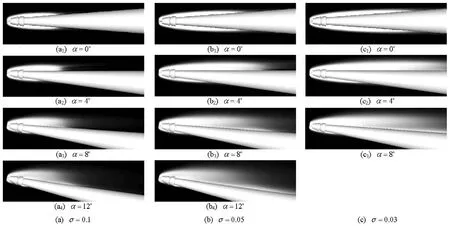
Fig.10 Flood contour of the numerically predicted cavities over the complex vehicle at various working conditions
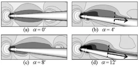
Fig. 11 Pressure contours showing the difference betweenthe two cavity situations (σ=0.05)
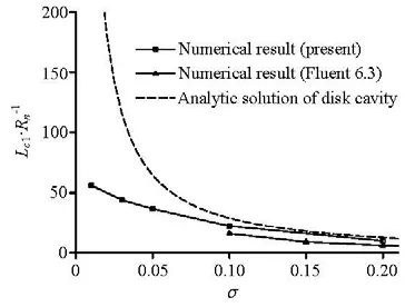
Fig.12 Axial length of the cavity Iowith relation to the changeof cavitation number (α=0)
Although the cavity scales have reflected some macroscopic character of the supercavity, the primarily concerned aspect about the submerged vehicle is its hydrodynamic properties, especiallythe drag-force. Cdis defined as Cd=Fd/(0.5ρπ), wheredenotes the radius of the cylinder. Figure 15 gives the predicted drag coefficients under various navigating conditions of the vehicle. The drag reduction effect of the cavity can be obviously observedwhen cavitation number is lowered, and similar reduction trend can be found for different angles of navigation pose. Additionally the angle has quite notable influence on the drag, which greatly rises when the vehicle is pulled up.
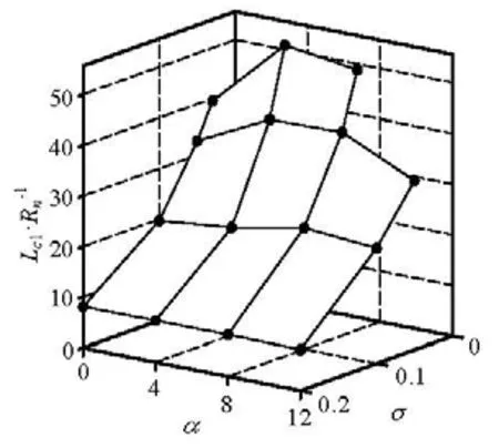
Fig.13 Axial length of the cavity I for various combinations of cavitation number and angle of attack
5. Conc lusion
In the numerical simulation methods, traditional linear eddy-viscosity turbulence modelscan not provide sufficiently accurate prediction for the cavitating flow which is accompanied with large density ratio and large-scaled swirling flow structure. Thequadratic and the cubic NLEVMs employed in the present workprovide better description for the anisotropic turbulence stresses, and were verified by benc hmark problem tobe able to obtain more accurate capture of the macroscopic and hydrodynamic properties of the cavitiesthan linear models. Accordingly, the non-linear models were further used to investigate the influence of vehicle’s profile on the shape and the drag. Ultimately, the cavitating flows around a particularly designed complex submerged vehicle have been numerically predicted with the application of the cubic model. The corresponding cavitation behaviors have been investigated in detail to provide a beneficial technological experience for further research.
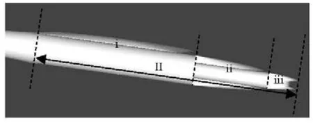
Fig.14 Configuration of the cavity of part II (=0.1σ,=α8o)
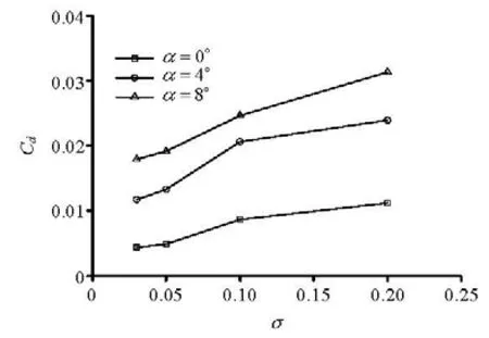
Fi g.15 Drag coefficients at different navigation conditions
[1]SAVCHENKO Y. Supercavitation–Problems andperspectives[C]. The 4th International Symposium on Cavitation. Pasadena, California, USA, 2001.
[2]VLASENKO Y. D. Experimental investigation of supercarvitation flow regimes at subsonic and tr ansonic speeds[C]. The 5th International Symposium on Cavitation. Osaka, Japan, 2003.
[3] MERKLE C. L., FENG J. Z. and BUELOW P. E. O. Computational modeling of the dynamics of sheet cavitation[C]. The 3rd International Symposium on Cavitation. Grenoble, France, 1998.
[4] QIN Q., SONG C. C. S. and ARNDT R. E. A. A numerical study of an unsteady turbulent wake behind a cavitating hydrofoil[C]. The 5th International Symposium on Cavitation. Osaka, Japan, 2003.
[5] BYEONG R. S., SATORU Y. and XIN Y. Application of preconditioning method to gas-liquid two phase flow computations[J]. Journal of Fluids Engineering, 2004, 126(4): 605-612.
[6] GONCALVES E., PATELLA R. F. Numerical simulation of cavitating flows with homogeneous models[J]. Computers and Fluids, 2009, 38(9): 1682-1696.
[7] KUNZ R. F., BOGER D. A. and STINEBRING D. R. et al. A preconditioned Navier-Stokes method for twophase flows with application to cavitation prediction[J]. Computers and Fluids, 2000, 29(8): 849-875.
[8] CHEN Ying, LU Chuan-jing. A homogenous-equilibrium-model based numerical code for cavitation flows and evaluation by computation cases[J]. Journal of Hydrodynamics, 2008, 20(2): 186-194.
[9] CHEN Ying, LUChuan-jing and WU Lei. Numerical method for three-dimensional cavitation flows at small cavitation number[J]. Chinese Journal of Computa- tional Physics, 2008, 25(2): 163-171(in Chinese).
[10] HEJRANFAR K., FATTAH-HESARY K. Assessment of a central difference finite volume scheme for modeling of cavitating flows using preconditioned multiphase Euler equations[J]. Journal of Hydrodynamics, 2011, 23(3): 302-313.
[11]SHAMS E., APTE S. V. Prediction of small-scale cavitation in a high speed flow over an open cavity using large-eddy simulation[J]. Journal of Fluids Engineering, 2010, 132(11): 111301.
[12]YUAN W., SAUER J. and SCHNERR G. H. Modeling and computation of unsteady cavitation flows in injection nozzles[J]. Mechanics and Industry, 2001,2(5): 383-394.
[13]SINGHAL A. K., ATHAVALE M. M. and LI H. Y. et al. Mathematical basis and validation of the full cavitation model[J]. Journal of Fluids Engineering, 2002, 124(3): 617-624.
[14] SAITO Y., NAKAMORI I. and IKOHAGI T. Numerical analysis of unsteady vaporous cavitating flow around hydrofoil[C]. The 5th International Sympo- sium on Cavitation. Osaka, Japan, 2003.
[15] OWIS F. M., NAYFEH A. H. Computations of the compressible multiphase flow over the cavitating highspeed torpedo[J]. Journal of Fluids Engineering, 2003, 125(3): 459-468.
10.1016/S1001-6058(11)60309-0
* Project supported by the National Natural Science Foundation of China (Grant Nos. 11102110, 10832007).
Biography: CHEN Ying (1979-), Male, Ph. D., Lecturer
杂志排行

水动力学研究与进展 B辑的其它文章
- REVIEW OF SOME RESEARCHES ON NANO- AND SUBMICRON BROWNIAN PARTICLE-LADEN TURBULENT FLOW*
- EFFECT OF A PROPELLER AND GAS DIFFUSION ON BUBBLE NUCLEI DISTRIBUTION IN A LIQUID*
- THE HYDRODYNAMIC CHARACTERISTICS OF FREE VARIABLEPITCH VERTICAL AXIS TIDAL TURBINE*
- NUMERICAL PREDICTION OF SUBMARINE HYDRODYNAMIC COEFFICIENTS USING CFD SIMULATION*
- SIMULATION OF OIL-WATER TWO PHASE FLOW AND SEPARATION BEHAVIORS IN COMBINED T JUNCTIONS*
- 3-D NUMERICAL SIMULATIONS OF FLOW LOSS IN HELICAL CHANNEL*