EFFECT OF A PROPELLER AND GAS DIFFUSION ON BUBBLE NUCLEI DISTRIBUTION IN A LIQUID*
2012-08-22HSIAOChaoTsungCHAHINEGeorges
HSIAO Chao-Tsung, CHAHINE Georges L.
DYNAFLOW, INC., Jessup, Maryland 20794, USA, E-mail: ctsung@dynaflow-inc.com
(Received December 26, 2011, Revised April 28, 2012)
EFFECT OF A PROPELLER AND GAS DIFFUSION ON BUBBLE NUCLEI DISTRIBUTION IN A LIQUID*
HSIAO Chao-Tsung, CHAHINE Georges L.
DYNAFLOW, INC., Jessup, Maryland 20794, USA, E-mail: ctsung@dynaflow-inc.com
(Received December 26, 2011, Revised April 28, 2012)
A multi-bubble dynamics code accounting for gas diffusion in the liquid and through the bubble wall was developed and used to study the modification of a bubble nuclei population dynamics by a propeller. The propeller flow field was obtained using a Reynolds-Averaged Navier-Stokes (RANS) solver and bubble nuclei populations were propagated in this field. The numerical procedure enabled establishment of the possibility of production behind the propeller of relatively large visible bubbles starting from typical ocean nuclei size distributions. The resulting larger bubbles are seen to cluster in the blade wakes and tip vortices. Parametric investigations of the initial nuclei size distribution, the dissolved gas concentration, and the cavitation number were conducted to identify their effects on bubble entrainment and the resultant void fractions and bubble distribution modifications downstream from the propeller. Imposed synthetic turbulence-like fluctuations unto the average RANS flow field were also used to study the effect averaging in the RANS procedure has on the results.
gas diffusion, bubble entrainment, propeller
Introduction
The generation and entrainment of bubbles by ship motion raises many two phase flow fundamental questions and is of interest as bubble generation could in hostile environments affect the safety of the ship. These bubbles are transported by the flow field to the stern area, captured in the ship wake, trapped in the large vortical structures, and then act as tracers of the ship wake. In littoral warfare, such bubbly wakes provide an excellent opportunity to homing devices enabling them to easily find their target because of the large acoustic cross sections and high acoustic response of bubbles to acoustic waves.
It is believed that bubble entrainment has two main sources. One source is from bubbles generated by air entrainment at the surface due to free surface and hull interactions resulting in breaking and spilling waves at the bow and stern and bubble entrainment in the boundary layer along the hull. The other potential source is bubble “production” by the propellers. While there have been some research efforts to understandand observe bubble generation and entrainment in breaking waves[1-4], much less has been done to investigate the second means of bubble generation/entrainment due to the propeller[5], which is investigated here.
One hypothesized scenario for generation and entrainment of bubbles by the propeller is rooted in the fact that natural waters always contain suspended microscopic bubble nuclei in addition to dissolved gas. These nuclei, when subjected to variations in the local liquid pressures, will respond dynamically by changing volume, oscillating, and eventually growing from sub-visual to become visible due to cumulative gas transfer into the bubbles. Several techniques have been used to measure the distribution and sizes of these nuclei both in the ocean and in laboratories. These include Coulter counter, holography, light scattering methods, cavitation susceptibility meters and acoustic methods such as the ABS ACOUSTIC BUBBLE SPECTROMETER®[6]. Franklin[7]had summarized some earlier nuclei size distribution measurements done by different researchers in different waters.
In order to investigate this type of bubble size enhancement, we have considered a numerical approach combining propeller flow filed viscous solution coupled with multi-bubble dynamics incorporation mode-ling of gas diffusion to account for the transfer of gases across the bubble walls. Such an approach has been summarized recently in Chahine[8]. 3DYNAFSDSM©is a Lagrangian multi-bubble tracking and dynamics code[9]using a bubble motion equation with a modified Rayleigh-Plesset bubble dynamics equation incorporating bubble Surface Averaged Pressures (SAP) to account for flow field non-uniformities, and a bubble slip velocity pressure term[10]. This numerical model allows consideration of the spatiotemporal variations of dissolved gas concentration around the bubble and enables full tracking of a realistic bubble nuclei population.
To investigate bubble “production” by a propeller, we have utilized this model to propagate a nuclei distribution in the flow field of a marine propeller (NSWCCD Propeller 5168). This flow field was simulated earlier by Hsiao and Pauley[11]using a Reynolds-Averaged Navier-Stokes (RANS) solver and validated with experimental measurements.
1. Numerical approach
1.1 Bubble dynamics model
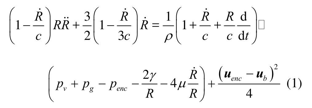
The dynamics of a spherical bubble has been extensively studied following the original works of Rayleigh[12]and Plesset[13]which included for an incompressible liquid, the effects of inertia, bubble content compressibility, and ambient pressure variations. Since then, a very large number of studies have been conducted to include a host of other physical phenomena. In the present study we have considered the following form of the equation for the bubble radius, R(t ), which accounts for liquid and gas compressibility, liquid viscosity, surface tension, and non-uniform pressure fields, and is based on Keller-Herring equation[14]. where c is the sound speed in the liquid,ρ its density, μ its viscosity, and pvits vapor pressure. pgis the pressure of the gas in the bubble, γ is the surface tension, and ubis the bubble travel velocity. In Eq.(1), which we dub the SAPbubble dynamics equation[9], we have accountedfor a slip velocity between the bubble and the host liquid, and for a nonuniform pressure field along the bubble surface.pencand uencare the liquid pressure and velocity respectively.pencand uencare defined as the averages of the liquid pressures and velocities over the bubble surface. The use ofpencresults in a major improvement over the classical spherical bubble model which uses the pressure at the bubble center in its absence. The gas pressure, pg, is obtained, as described in the next section, from the solution of the gas diffusion problem and the assumption that the gas is an ideal gas.
The bubble trajectory is obtained using the following motion equation
where ρbis the air density, CDis the drag coefficient given by an empirical equation from Haberman and Morton[15]and Ω is the deformation tensor. The 1st right hand side term is a drag force. The 2nd and 3rd terms account for the added mass. The 4th term accounts for the presence of a pressure gradient, while the 5th term accounts for gravity and 6th term is a lift force.
1.2 Gas diffusion model
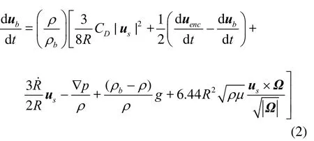
Water can contain gas not only in the form of nuclei with a particular distribution, but also as a gas dissolved in the liquid with a concentration C Over time, dissolved gas will diffuse from high concentration regions into low concentration regions following a gas transport equation for the time and space dependent dissolved gas concentration, C(x,t ), given by
wheregD is the molar diffusivity of the gaseous component in the liquid (in practice the turbulent diffusivity in high turbulence areas).
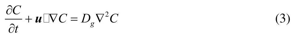
For an oscillating bubble in a liquid containing dissolved gas, Eq.(3) needs to be solved while satisfying the following initial and far field boundary conditions:
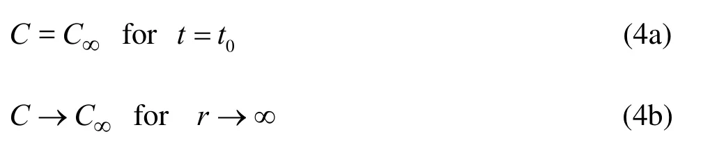
where ris the radial distance from the bubble center and C∞is the dissolved gas concentration far away from the bubble surface.
At the bubble surface Henry’s law, which relates the concentration of gas in a liquid to the partial pressureof the gas above the liquid, applies. Hence, we have at r=R
whereH is the Henry constant.
As the bubble oscillates, non-condensable gas is transported across the bubble wall. The rate of transport of gas moles into the bubble, n˙g, can be related to the gradient of gas concentration in the liquid at the bubble wall
where Sis thesurface of the bubble, ∂C/∂n is the normal derivative to the bubble surface of the liquid gas concentration. The integration on the handside of Eq.(6) is over the bubble surface. Time integration of Eq.(6) determines at every instant the total number of moles of gas, ng, in the bubble.
The two components of the bubble content: vapor and gas, are both assumed to b e ideal gases which follo w an ideal gas law
where Vbis the volume o f bubble, pvis the vapor pressure,nvis number of moles of vapor within the bubble, Ruis the universal gas constant and Tbis the absolutetemperature of the gas and vapor mixture. Due to therelatively short vaporization time compared to bubble dynamics and gas diffusion characteristic times, the vapor is considered to instantaneously flow in and out of the bubble, and pvis taken equal to the equilibrium vapor pressure of the liquid at the bubble wall temperature. One consequence of this assumption is that the amount ofng, and nvin the bubble are directly proportional to the ratio of their respective partial pressures.
Use of the idea gas equation of state introduces another unknown Tb. This problem can be closed by considering the thermodynamics of the contents of the bubble using the first law energy balance of the ideal gas mixture within the bubble. We consider the bubble wall to constitute a deformable and permeable control surface and write the first law energy balance for the control volume bounded by that surface
where dUis the change in internal energy, dW is the work done on the control volume, hiis the specific enthalpy, cVis the specific heat at constant volume, cPis the specific heat at constant pressure and Tiis the liquid temperature.
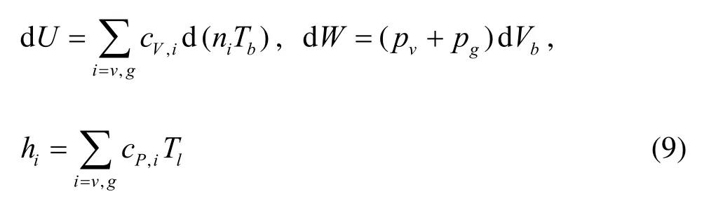
Combining Eq.(8) and (9) one can obtain
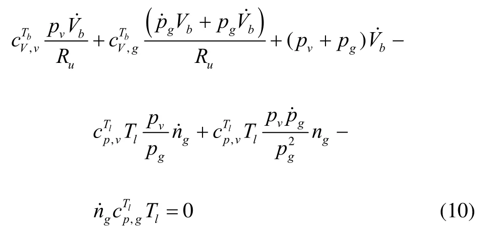
where the superscripts Tband Tlfor cVand cPindicate that the specificheats are evaluated at corresponding bubble or liquid temperature. Using the fact that cP-cV=Ruone can rearrange Eq.(10) to become:
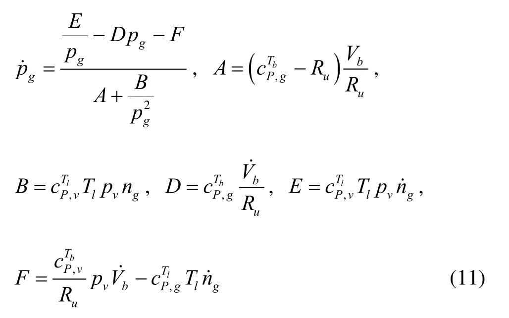
Integration of Eq.(11) provides the instantaneous gas pressure to be used in Eq.(1) and the boundary condition, Eq.(5).
A general, detailed solution of Eq.(3) would involve a time consuming numerical procedure, such as a space and time dependent finite difference scheme.To avoid this, an d since we want to consider very large number of nuclei/bubbles, we adopt the thin boundary layer approximation introduced by Plesset and Zwick[16]to obtain a solution to Eq.(3) for the case of an isolated spherical bubble. In this approach large gradients in gas concentration are concentrated in a bubble wall boundary layer which is small compared to the bubble radius. An analytical solution then exists and relates the gas concentration at the bubble wall to the concentration at “infinity”. This expression requires integration over the whole history of the bubble dynamics in order to enable computation of the amount of gas inside the bubble, and has the following form
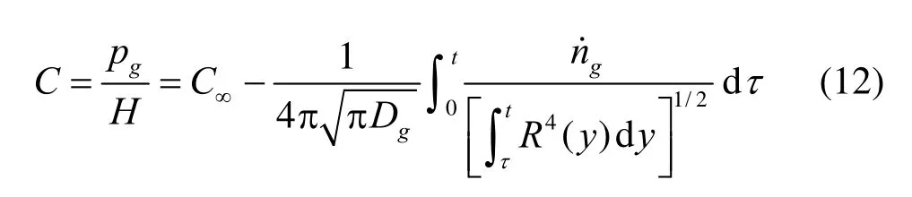
Although solving Eq.(12) instead of Eq.(3)reduces numerical complexity, some loss of solution generality is expected due to the thin layer approximation and the neglect of convection term.
Equation (11) requiresgn andto be integrated in time. To do so we rewrite Eq.(12) by first assigning the time interval integration part to be
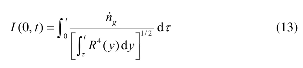
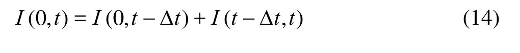
The interval time integration[0,t] can be split into two intervals to separate out the current time step as
where Δt is the time step size. The second terms in Eq.(14) is evaluated analytically to avoid the (tτ)-1/2sing ularity att=τ
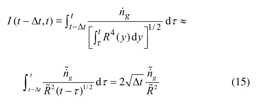
where the tildes denote average values over the interval [t-Δt,t]. If we approximatethese average vales by≈(t)and≈[R(t)+R(t-Δt )]/2, then Eq.(15) becomes
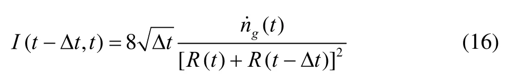
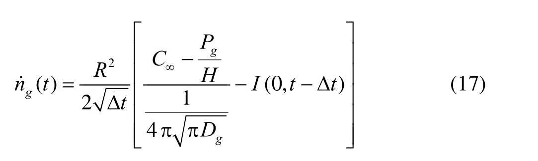
After substituting Eq.(17) and (13) into Eq.(15), we can rearrange Eq.(15) to become
To determine each bubble motion andvolume variation, the set of four differential Eq.(1), (2), (12) and (18) are solved using a Runge-Kutta fourth-order scheme to integrate through time.
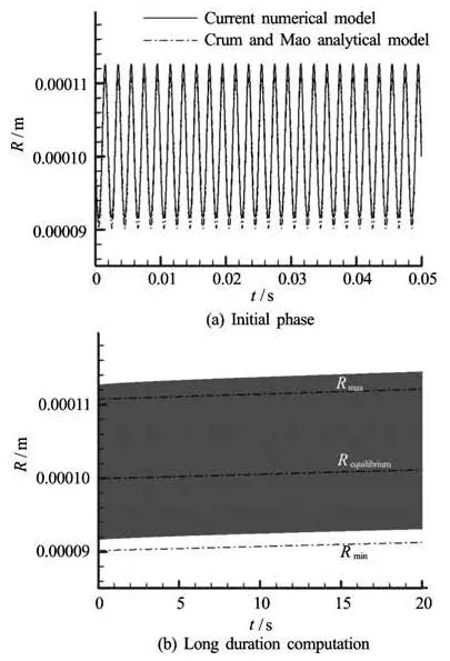
Fig.1 Comparison of bubble radius versus time and resulting bubble growth from rectified diffusion between the current numerical model and Crum and Mao’s analytical model[17]
The current numerical model is compared to the analytical model derived by Crum and Mao[17]for a rectification diffusion bubble driven by an acoustic pressure field as shown in Fig.1. It is seen that the comparison between our current numerical model and Crum’s analytical model shows a good agreement on the bubble growth rate except at the very beginning. Also, due to the neglect of all but the first-order term in the Crum analytical model, the bubble maxima andminima of the analytical model are seen to be a few percent smaller than in the present numerical model.
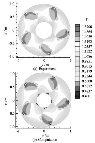
Fig.2 Axial velocity Vxfrom experiment and computationat x/Rp=0.2386
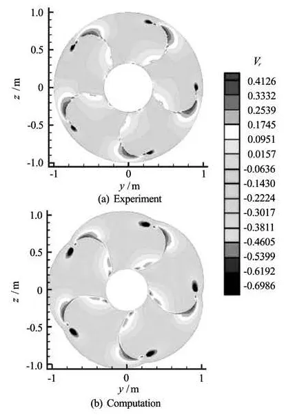
Fig.3 Radial velocity Vrfrom experiment and computation at x/Rp=0.2386
2. Results and discussion
The above method was applied to study nuclei motion and size variations in a selected propeller flow field. Nuclei in natural water with a prescribed air void fraction were releasedupstream of a rotating propell©er and their dynamics computed using 3DYNAFSVIS. The propeller model was the David Taylor Propeller 5 168 propeller which is a five-blade propeller with a 15.856 inch (0.4 m) diameter. The flow field around this propeller was simulated earlier for three different advance coefficients by Hsiao and Pauley[11]using a RANS solver and were validated against experimental measurements conducted by Chesnakas and Jessup[18]. Figure 2 and Fig.3 illustrate the good comparison between simulation and measurement for the axial and radial components of velocity field. Additional more detailed comparisons can be found in Hsiao and Pauley[11]. The propeller flow field condition used in the study corresponded to an advance coefficient J=U∞/nD =1.1, where the liquid velocity U∞=10.7 m/s, the propeller number of revolutions per minutes, n=1 450 rpm, and D=0.4 m the propeller diameter.
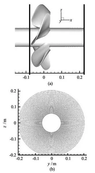
Fig.4 Release location of the nuclei upstream from the rotating propeller for the “synthetic” case study presented here to illustrated effect of propeller on nuclei space and size distribution
3. Gas diffusion effects
To study t he gas diffusion effects on the bubbledynamics and the size distribution downstream from the propeller, we compare the results for a “synthetic”bubble nuclei distributionof including or not gas diffusion effects. Nuclei with a uniform radius of 50 μm were released from a preset grid located upstream from the propeller at x=–0.08 m as illustrated in Fig.4. The total number of nuclei released was 4 500 and the nuclei were tracked from x=–0.08 m to x= 0.3 m. For the computations with gas diffusion, the water was assumed to be saturated with gas (i.e., the dissolved gas concentration was 100%, i.e., C= 0.66 mol/m3).
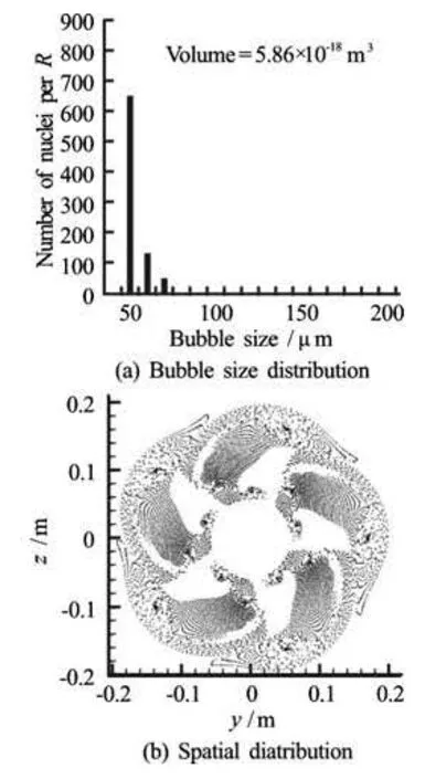
Fig.5 Bubble size and location distribution at theexit of the computational domain for simulations without gas diffusion at the exit from the computational domain,x= 0.22 m
Figure 5 and Fig.6 show the resulting bubble size andspatial distributions at x=0.22 m. for thetwo conditions where gas diffusion was not taken into account (Fig.5) and where itwas (Fig.6). These simulations were conducted at a cavitation number, σ= 1.75, where σ is defined as
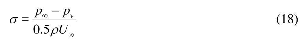
where p∞and pvare the liquid pressure and velocity upstreamfrom the propeller.
From the comparison of the bubble size distributions it is seen that the propeller modifies the size range of the bubbles from the uniform 50 μm nuclei sizes to a range of sizes: 50μm<R<70μm when therewas no gas diffusion. When gas diffusion is taken into account a much larger range of bubble sizes is generated: 50μm<R<190μm . In both cases larger sized bubbles are seen to coll ect mainly in two regions: the tip vortices areas and the wakes of the blades, which emanate from its blade suction side.
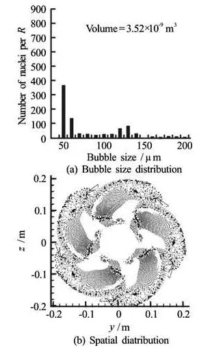
Fig.6 Bubble size and location distribution at theexit of the computational domain for simulations withgas diffusion at the exit from the computational domain, x=0.22 m
By observing the behavior of individual bubbles, we are able to determine where the larger bubble originated from. Figure 7 shows three typical scenarios of bubble paths through the propeller flow field.
(1) In the first (Fig.7(a)) the bubble has a helicoidal motion and gets entrapped in a tip vortex. It grows to its maximum size while approaching the vortex core and feeling the lowest pressure region. The bubble then shrink in volume while oscillating as the pressure along the vortex center recovers. However, the bubble does not return to its initial size (50 μm), instead it retains a much larger size (80 μm) due to a net increase of the amount of gas in the bubble accumulated during the volume fluctuations.
(2) In the second scenario, the bubble travels over the blade surface on the suction side (Fig.7(b)). Here the bubble grows to its maximum size as it encounters the minimum pressure on the blade surface. It then collapses as the pressure recovers, but here again retains a much larger size (110 μm) than the original after it passes the blade area.
(3) The third scenario is the most common, and concerns bubbles passing through the blade areas away from the tip vortices and blade suction side regions. For these bubbles the size remains very close to the original size during and after crossing the prope-ller f low field, as shown in Fig.7(c).
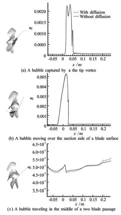
Fig.7 Bubble trajectories along the propeller and bubble radius along the trajectories
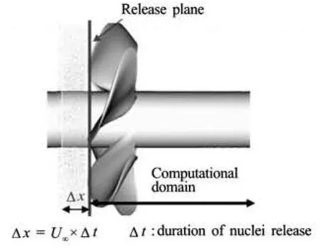
Fig.8 Illustration of the fictitious volume used to feed nuclei into the inlet (or release area) of the computational domain
4. Modeling of a real nuclei field
In order to simulate realistic water conditions a known size distribution of nuclei was selected and used toseed the water feeding the propeller. The nuclei were considered to be distributed randomly in a fictitious supply volume feeding the computational domain inlet plane (release area). The fictitious volume size was determined as the product of the release area by the sought physical duration of the simulation and the inlet velocity, U∞, as illustrated in Fig.8. The nuclei size density distribution function, n(R), is defined as the number of nuclei per unit volume having radii in the range[R,R+dR]
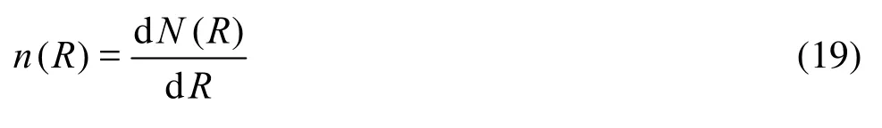
where N(R) is the number of nuclei of radiu s R in aunit volume. This function can be expressed as a discrete distribution of M selected nuclei sizes. Thus, the total void fractio n, α, in the liquid can be obtained from
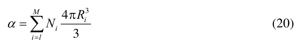
where Niis the discrete number of nuclei of radius Riused in the computations.
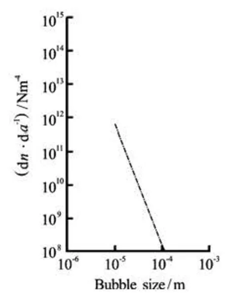
Fig.9(a)Thenuclei size density distribution selected to resemblethefield measurement byMedwin[7]
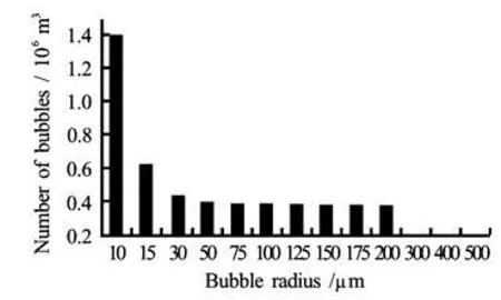
Fig.9(b) The resultant number of nuclei released
For the results shown below we have selected the following characteristic values, which correspond to typical field measurement by Medwin[7]size range of 10 μm to 200 μm and void fraction, α=3.23×10⁻⁵. Figure 9(a) shows the selected nuclei size numberdensi ty and Fig.9(b) shows the numbers of discrete bubble sizes and bandwidths selected.
5. Time-Averaged void fraction distribution
In order to minimize computations CPU time, a time of release, Δt, during which actual bubble compu tations are conducted was selected and correspond ed to a meaningful bubble population distribution in the fictitious bubble supply volume. The resulting bubble behavior was then assumed to be repeated for mΔt and the effects of m on the results were analyzed.
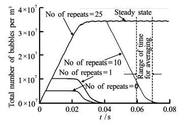
Fig.10Effect of the bubble release duration on the total number of bubbles within the computational domain. Computations were conducted for Δt=3.7×10⁻³s and results were then repeated to cover much longer release times, mΔt,m=1-25
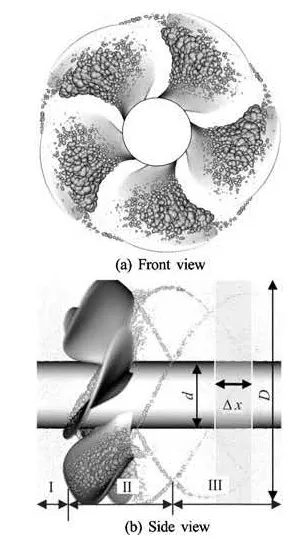
Fig.11 Snapshot of the bubbles in the propeller flow field of the bubbles in the computational domain ata given time during the computation. Bubble sizes are to-scale in volume II, they are enhanced by a factor of5 in the volumes I and III
Figure 10 shows the time variation of the total number of bubbles within the computational domain (-0.08m<0.3m) for Δt=3.7×10⁻³s and for different number of repeats, m. The results clearly indicate that a steady sta teis achieved after t>0.03 ms whena minimum of 10 repeats is effectuated. For a smaller value of the release duration the solution is only transient. Increasing the number of repeats, m, over 10 extends the quasi-steady state period in the computational domain.
Figure 11 illustrates the sizes and locations of the bubbles on the propeller blades and in the tip vortices. A snapshot of both front and side views are shown for σ=1.75. It is noted that in the side view the bubbles in the volume II are shown to scale, while they are amplified 5 times (to make them more “visible” in print) in the volumes I and III. Figure 11 illustrates the marked increase in “visible” bubbles downstream of thepropeller, traveling bubble cavitation, tip vortex cavitation and the initiation of sheet cavitation.
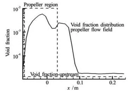
Fig.12 The distribution of the time-averaged void fraction,, along the propeller axialdirectionfor avalueof void fraction at the inlet, α=3.23×10⁻⁵and α=1.75
In order to illustrate the results in a simp lified manner, some average quantities are introduced. We can define a section-averaged time dependent void fraction, αΔx(x,t), as follows
where d is the shaft diameter,D, the propeller diameter,and N(x,t)is the number of bubble within the interval [x,x+Δx]at thegiven time, t. The time-averaged void fraction ofα(x,t)att1, over a time period dt can also be defined as
Figure 12 shows the distributionofαalong x. It is seen thatthe void fraction increases significantly as a result ofcavitation on the blades (first hump in the figure) and in the tip vortices (second hump). The void fraction decreases asthe pressure encountered by the bubble increases. However, the downstream void fraction is in this case still becomes 1.4 times that of upstream.
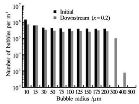
Fig.13 Comparison of the initial nuclei size distributionentering the computational domain and that resulting at the domain exit at x=0.2 m
The effect of propeller cavitation on the number of bubbles having a large size is much more important than on. Figure 13 shows the bubble size distribution at x=0.2 m. It is seen that a large number of bubbles of 400 μm radius are now present in the field and would be seen, while all bubbles were originally smaller than 200 μm upstream when they entered the propeller flow field.
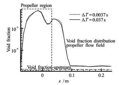
Fig.14 Comparison of the time-averaged void fraction distribution,, along the axial direction between two different durations of the nuclei release
6. Effect of the duration of nuclei release
In order to investigate whether the duration of bubble release selected in the previous section, Δt= 3.7×10⁻³s, is long enough to be statistically meaningful, comparison with a computation with a 10fold longer release time, Δt=3.7×10⁻²s is considered here. Comparison ofthe void fractionsαisshown in Fig.14. It is seen that differences between the two release durations are minimal with less than 2.5% difference in the time-averaged void fraction downstream. This justifies the use of the shorter duration of 3.7×10⁻³s to conduct parametric studies.
7. Parametric studies
The effect of three important physical parameters: the cavitation number, the initial nuclei size distribution, and the initial dissolved gas concentration, on the bubble nuclei entrainment and dynamics are addressed in this section.
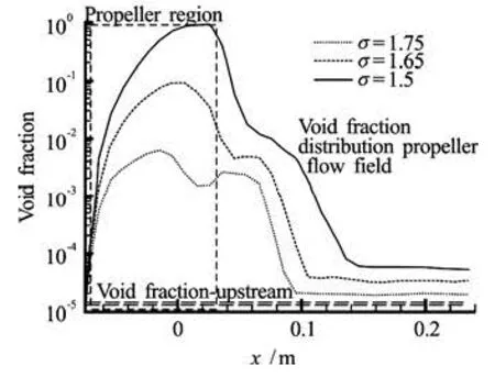
Fig.15Comparison of the void fraction variations along x for three cavitation numbers, σ=1.75, 1.65 and 1.5
7.1Cavitation number
The time-averaged void fraction and downstream nucleisize distribution obtained at three different cav itation numbers, σ=1.5, 1.65 and 1.75, are compared in Fig.15 and Fig.16. As can be seen in the figures, in all three cases the voidfaction increases significantly inthe propeller liquid volume II (Fig.11(b)), th en plateaus. As the cavitation number decreases, the void fractions within the cavitation areas increase and the relative importance of the tip vortices cavitation volume diminishesrelative to the propeller blade cavitation. With smaller values ofσ, the bubbles retain a much larger size downstream of the propeller due to enhanced net gain of gas mass diffusing into the bubbles. The downstream void fractionαatx=0.2 m is 50 times the upstream value for σ=1.5, 2.35 times for σ=1.65 and 1.4 times for σ=1.75. The largest downstream bubble radii observed are 800 μm for σ=1.5, 600 μm for σ=1.65 and 400 μm for σ=1.75, as compared to 200 μm at release.
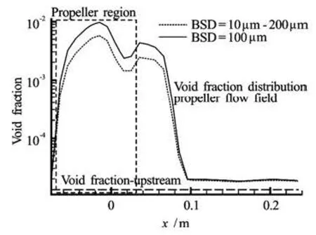
Fig.17 Comparison of the void fraction variation along the propeller streamwise direction for two initial nuclei size distributions
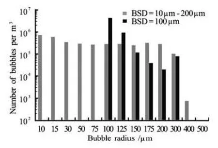
Fig.18 Bubble size distribution at x=0.2 m for two initial nuclei size distributions
7.2Nuclei distribution
To investigate the effect of the initial nuclei size distribution on the results a bubble size distribution ranging from 10 μm-200 μm is compared in Fig.17 to thatof a uniform distribution of 100 μm bubbles.Both distributions are selected to have the same initial void fraction. Figure 17 showsα(x) in both cases. Higher bubble void fractions are seen near the propeller blade region for the initial uniform nuclei size case. However, this does not result in any significant difference in the void fraction observed downstream. Figure 18 compares the resulting downstream nuclei size distributions at x=0.2 m. It is seen that the largest bubble radius is 400 μm for the non-uniform nuclei distribution, while it is 300 μm for the uniform case. This is related to the existence of larger bubbles in the initial non-uniform bubble nuclei distribution.
7.3 Dissolved gas concentration
The effect of the dissolved gas concentration on the bubble dynamics is illustrated in Fig.19 by c3onsidering disso3lved gas concentration of 0.66 mol/m and 1.32 mol/m. As seen in Fig.19, this results in further increase in the void fraction downstream. However, although the dissolved gas concentration was doubled, the void fraction increased by only 11%.
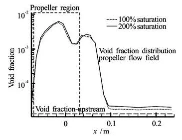
Fig.19Comparison of the void fraction variation along the propeller streamwise direction for two initial gas concentrations
8. Eff ect of artificial turbulence-like fluctuations
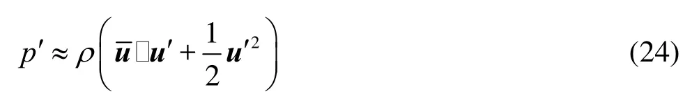
The computations shown above used the flow field obtained by a RANS computation.As a result, the pressures and velocities used were quantities averaged by the RANS numerical procedure. On a real propeller, fluctuating turbulent quantities exists and modulate the RANS solution. In order to investigate the influence of turbulence on the results shown above, artificial turbulence-like fluctuations, (u',p'), were randomly added to the velocity and pressure field, (,), obtained from RANS

To reproduce a realistic turbulent flow, the fluctuation velocity field, u', was composed of both spatial and temporal fluctuations. The pressure fluctuation field were then approximated by
The following expressions give the fluctuating velocity field for theaxial component only (for simplicity of the presentation):
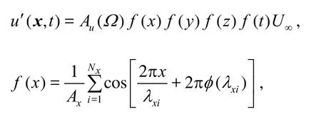
To make the artificial fluctuations physics-based, their intensity Au(Ω)was related to the RANS determined vorticity distrib ution, Ω, andmade maximum at
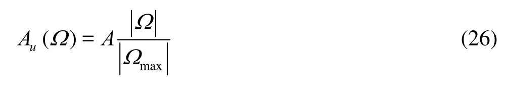
where A is the imposed amplitude of the oscillations and Ωmaxis the maximum vorticity in a given y-z plane.
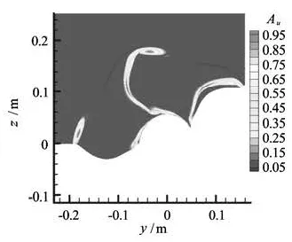
Fig.20 Contour plots of the imposed velocity fluctuations amplitude Au(Ω) in the y-z plane located at x= 0.05 m
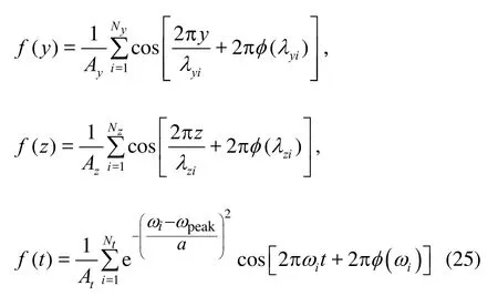
Figure 20 illustrates the contours of Au(Ω)in the y-z plane downstream of the propeller at x= 0.05 m.Two flow passages only of the five-bladed propeller are shown. As expected, the highest amplitude oscillations are in the tip vortices and along the wake regions of the propeller blades. In Eq.(25), f(x), f(y)andf(z) are spatial fluctuation functions, madeofΝx, Νyand Νzcomponents with wave lengths and phases, λxand φ(λx), λyand φ(λy), λz, and φ(λz) respectively. The phase shiftsφ are randomly distributed between [0,1]. Ax, Ayand Azare factors used to ensure that the fluctuation functions have unit values at the highest oscillations amplitude.
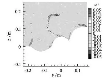
Fig.21 Contour plots of the axial velocity fluctuations obtained with A=0.05 and composed of 400 different wave lengths ranging from 0.001 m to 1 m in boththey and z direction
By multiplying f(x), f(y) and f(z )with Au(Ω), one can obtain the spatial velocity field fluctuations. The axial velocity fluctuation co ntours shown in Fig.21 were obtained with A=0.05 and 400 wave lengths ranging from 1 m to 0.001 m in both the y and z directions.
Fig.22 Example fluctuations function with ωpeak=8 kHz, and composed of frequencies between 1 kHz and 15kHz
Equation (25) also includes an imposed temporal fluctua tion, f(t), which is composed of Ntdiffe-re nt frequencies,ω, with phase shift φ(ω)randomly distributed between [0,1]. At is afactor to ensure that the fluctuation function has a unit value at the highest amplitude of oscillations. The exponential term included in the temporal function allows one to generate bias fluctuations with the highest energy centered in the specified peak frequency, ωpeak. Figure 22 illustratesanexample signal composed of frequencies between 1 kHz to 15 kHz with ωpeak=8 kHz shown in both the time and frequency domains.
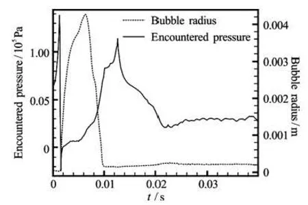
Fig.23 Encountered pressure (black) and bubble radius (grey) for a 50 μm nuclei which grew over a propeller blade suction surface, σ=1.75
With this imposed artificial turbulence, weinvestigate the effects of the fluctuations amplitudeand frequency on the bubble dynamics and entrainment. Figure 23 shows in black the bubble encountered pressure (i.e., pressure felt by the bubble during its travel) and in grey the bubble radius versus time for a 50 μm bubble in absence of imposed fluctuations. This bubble grew to more than 0.004 m near a blade surface and then stabilized to ab out 200 μm downstream ofthe propeller. The cavitation number was σ= 1.75.
Figure 24 shows similar curves as in Fig.23 but when artificial turbulent flow field like fluctuations were imposed. The results for three conditions are shown in the figure with different peak frequencies: ωpeak=2 kHz, 6 kHz and 10 kHz and A=0.4. It is clear from the figures that the bubble has the strongest oscillations and the largest downstream radius when the peak frequency is equal to 6 kHz. This can beexplained by considering the bubble natural frequency, ωR, given by
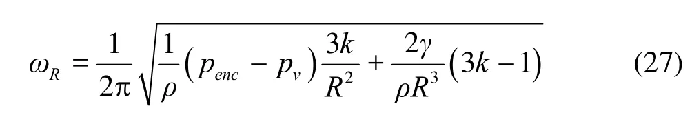
where k is the polytrophic gas constant (=k1.4 was used in the current study). Not surprisingly, for the bubble shown in Fig.23, the natural oscillation frequencyis about 6 kHz since it has a radius of 200 μm and encounters a pressure of around 30 000 Pa. As expected, oscillations with a driving pressure field resonating with the bubble natural frequency enhance the gas diffusion. This resonating oscillations are expected to increase further the size of the resulting bubble as we have shown in Fig.1.
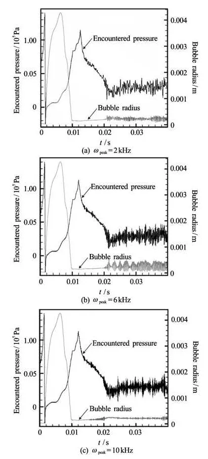
Fig.24 Encountered pressure (black) and bubble radius (grey) for a 50 μm nuclei subjected to imposed artificial flow field fluctuations with three different peak frequencies, ωpeak=2 kHz, 6 kHz and 10 kHz, A=0.4
Also, the effect of the amplitude of the fluctuations on the results is shown in Fig.25 for threedifferent values of the amplitude,A, and with ωpeak= 6kHz. As expected, the bubble oscillations increase when the amplitude of the fluctuations increases.
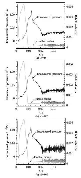
Fig .25 Encountered pressure (black) and bubble radius (grey) for a 50 μm nuclei subjected to imposed artificial flow field fluctuations with three different fluctuation amplitudes: A=0.1, 0.2 and 0.4, ωpeak=6 kHz
9.Conclusions
Application of multi-bubble dynamics, accounting for gas diffusion effects to the study of bubble entrainment and dynamics in a propeller flow enables studyof the modification of natural waters nuclei distribution by a propeller. Comparison of the results between inclusion or neglect of gas diffusion shows that gas diffusion plays an important role on the resulting bubble sizes downstream from the propeller. Bubble sizes become larger than the original upstream sizes, downstream of the propeller due to a net influx of dissolved gas into the bubble. Bubble explosive stream void fraction. Different upstream nuclei distributions with the same void fraction have similar effegrowth and collapse, are also seen to be an essential“catalyst” to enable significant diffusion as bubbles which do not experience intense dynamics do not change size significantly.
The model enabled simulations of bubble entrainment by a rotating propeller with a realistic ocean nuclei size distribution. Large visible bubbles were seen to collect in the blades vortices and wake regions. As the cavitation number decreases the downstream void fraction increases and the nuclei size distribution shifts towards larger sizes. Increase in dissolved gas concentration was also found to increase the downcts on the downstream void fraction but have a more significant effect on the downstream nuclei size distribution. Changes in the bubble size are indeed the most important effect observed in the study, with the propeller flow field significantly modifying the size distribution by both broadening the size range and increasing significantly the number of larger bubbles.
Imposing artificial turbulence on the flow field results in enhanced bubble activity, which increases with the fluctuations amplitude. The magnitude of the bubble size oscillations reaches a maximum as the peak frequency of the imposed turbulent fluctuations matches the resonant natural bubble oscillation frequency.
Acknowledgements
This work was conducted at Dynaflow, Inc. (www.dynaflow-inc.com) and was supported by the Office of Naval Research (Grant No. N00014-05-C-0170) monitored by Dr. Patrick L. Purtell. We would also like to thank Dr. Kim Ki-Han at ONR for his support of this program.
[1] RAICHLEN F. A., BRENNEN C. E. Measurement of air entrainment by bow waves[J]. Journal of Fluids Engineering, 2001, 123(1): 57-63.
[2] DUNCAN J. H. Spilling breakers[J]. Annual Review of Fluid Mechanics, 2001, 33: 519-547.
[3] MUSCARI R., MASCIO A. D. Numerical modeling of breaking waves generatedby a ship’s hull[J]. Journal of Marine Science and Technology, 2004, 9(4): 158- 170.
[4] MORAGAF. J., CARRICA P. M. and DREW D. A. et al. A sub-grid air entrainment model for breaking bow waves and naval surface ships[J]. Computes and Fluids, 2008, 37(3): 281-298.
[5] PEREIRA F. Transport of gas nuclei in a propeller[C]. Second International Symposium on Marine Propu- lsors SMP’11. Hamburg, Germany, 2011.
[6] WU Xiong-jun, CHAHINE Georges L. Development of an acoustic instrument for bubble size distribution measurement[J]. Journal of Hydrodynamics, 2010, 22(5
Suppl.): 330-336.
[7] FRANKLIN R. E. A note on the radius distribution function for microbubbles of gas in water[C]. ASME Cavitation and Multiphase Flow Forum. Los Angeles, California, USA,1992, 77-85.
[8] CHAHINE Georges L. Numerical simulation of bubble flow interactions[J]. Journal of Hydrodynamics, 2009, 21(3): 316-332.
[9] HSIAO C.-T., CHAHINE G. L. Scaling of tip vortex cavitation inception noise with a statistic bubble dynamics model accounting for nuclei size distribution[J]. Journal of Fluid Engineering, 2005, 127(1): 55-64.
[10] HSIAO C.-T., CHAHINE G. L. and LIU H.-L. Scaling effects on prediction of cavitation inception in a line vortex flow[J]. Journal of Fluid Engineering, 2003, 125(1): 53-60.
[11] HSIAO C.-T., PAULEY L. L. Numerical computation of the tip vortex flow generated by a marine propeller[J]. Journal of Fluids Engineering, 1999, 121(3): 638-645. [12] RAYLEIGH L. On the pressure developed in a liquid during collapse of a spherical cavity[J]. Philosophical Magazine Series 6, 1917, 34(200): 94-98.
[13] PLESSET M. S., DAVIES R. Cavitation in real liquids[M]. Elsevier Publishing Company, 1964, 1-17.
[14] VOKURKA K. Comparison of Rayleigh’s, Herring’s, and Gilmore’s models of gas bubbles[J]. Acustica, 1986, 59(3): 214-219.
[15] HABERMAN W. L., MORTON R. K. An experimental investigation of the drag and shape of air bubbles rising in various liquids[R]. Report 802, DTMB, 1953.
[16] PLESSET M. S., ZWICK S. A. A non-steady heat diffusion problem with spherical symmetry[J]. Journal of Applied Physics, 1952, 23(1): 95-98.
[17] CRUM L. A., MAO Y. Acoustically enhanced bubble growth at low frequencies and its implications for human diver and marine mammal safety[J]. Journal of the Acoustical Society of America, 1996, 99(5): 2898- 2907.
[18] CHESNAKAS C., JESSUP S. Experimental characterization of propeller tip flow[C]. 22th Symposium on Naval Hydrodynamics. Washington D.C., 1998, 156-170.
10.1016/S1001-6058(11)60308-9
* Biography: HSIAO Chao-Tsung (1964-), Male, Ph. D., Principal Research Scientist
杂志排行

水动力学研究与进展 B辑的其它文章
- REVIEW OF SOME RESEARCHES ON NANO- AND SUBMICRON BROWNIAN PARTICLE-LADEN TURBULENT FLOW*
- APPLICATION OF QUADRATIC AND CUBIC TURBULENCE MODELS ON CAVITATING FLOWS AROUND SUBMERGED OBJECTS*
- THE HYDRODYNAMIC CHARACTERISTICS OF FREE VARIABLEPITCH VERTICAL AXIS TIDAL TURBINE*
- NUMERICAL PREDICTION OF SUBMARINE HYDRODYNAMIC COEFFICIENTS USING CFD SIMULATION*
- SIMULATION OF OIL-WATER TWO PHASE FLOW AND SEPARATION BEHAVIORS IN COMBINED T JUNCTIONS*
- 3-D NUMERICAL SIMULATIONS OF FLOW LOSS IN HELICAL CHANNEL*