Situational continuity-based air combat autonomous maneuvering decision-making

Jin-dong Zhng ,Yi-fei Yu ,Li-hui Zheng ,b ,Qi-ming Yng ,Guo-qing Shi ,* ,Yong Wu

a School of Electronics and Information, Northwestern Polytechnical University, Xi'an, 710129, China

b Military Representative Office of Haizhuang Wuhan Bureau in Luoyang Region, 471000, China

Keywords: UAV Maneuvering decision-making Situational continuity Long short-term memory (LSTM)Deep Q network (DQN)Fully neural network (FNN)

ABSTRACT In order to improve the performance of UAV’s autonomous maneuvering decision-making,this paper proposes a decision-making method based on situational continuity.The algorithm in this paper designs a situation evaluation function with strong guidance,then trains the Long Short-Term Memory (LSTM)under the framework of Deep Q Network (DQN) for air combat maneuvering decision-making.Considering the continuity between adjacent situations,the method takes multiple consecutive situations as one input of the neural network.To reflect the difference between adjacent situations,the method takes the difference of situation evaluation value as the reward of reinforcement learning.In different scenarios,the algorithm proposed in this paper is compared with the algorithm based on the Fully Neural Network (FNN) and the algorithm based on statistical principles respectively.The results show that,compared with the FNN algorithm,the algorithm proposed in this paper is more accurate and forwardlooking.Compared with the algorithm based on the statistical principles,the decision-making of the algorithm proposed in this paper is more efficient and its real-time performance is better.

1.Introduction

UAVs have the advantages of light weight,small size,strong maneuverability,and no fear of damage.In the future,they will gradually become the main force in the field of air combat [1].Autonomous air combat will be the final form of UAVs participating in air combat [2].However,the uncertainty and incomplete observability of the air combat environment and the high maneuverability of enemy fighters have put forward higher requirements for the real-time and efficiency of UAV decision-making.Air combat capability is of great significance [3].Autonomous maneuvering decision-making refers to the process in which the UAV autonomously generates control instructions for the aircraft based on past experiences and current air combat situation [4].There are many mature solutions to the maneuver decision-making problem in one-on-one air combat scenarios,which can be roughly divided into three categories: strategy-based methods [5],optimization algorithm-based methods,and artificial intelligence-based methods.

Strategy-based decision-making methods such as game theory method[4],[6],[7],[8],[9]and influence diagram method[10].The maneuver decision-making method based on game theory includes matrix gaming method and differential gaming method [8].The matrix gaming method can take into account various factors in the confrontation,but its state space is discrete,and due to the limitation of the algorithm,it cannot produce a decision result that considers the long-term benefits[7];The differential game method can conduct a comprehensive and systematic analysis of the object,but the calculation amount is too large when applied to a complex air combat model.The influence diagram method can reflect the pilot's decision-making process and consider the uncertainty of the environment [5],but it is difficult to obtain reliable prior knowledge in practical applications.There are many methods based on optimization algorithms,such as Genetic Algorithms[11]Bayesian Networks[12]and Rolling Time Domain Optimization[13].Among them,the genetic algorithm [14]can generate continuous and stable control variables,but the real-time performance of solving large-scale problems is too poor to be used in online air combat;The article[12,15]uses Bayesian reasoning to divide the air combat into four situations,but it does not consider the impact of the speed factor on the air combat situation;The paper [13]regards the maneuvering decision problem as a rolling time domain control problem,and proposes an optimization algorithm TSO with good robustness.

AI-based decision-making methods include expert system method[16],[17],[18]artificial neural network method[19,20]and reinforcement learning method.The expert system method utilizes existing air combat knowledge to handle the air combat situation for decision making[18],but with the increasing uncertainty of air combat,past experiences is not sufficient to handle all air combat scenarios;The artificial neural network method[21]relies on many data samples to train the neural network.This method has strong robustness,but the quality of the air combat samples will greatly affect the training effect;Compared with the neural network method,the reinforcement learning method can explore the environment by itself to obtain training samples,so the existing research mostly uses DQN to train the neural network.

The decision-making method based on reinforcement learning has problems such as discontinuous action space,insufficient guidance of the situation evaluation function,and difficulty in convergence of network training.Aiming at the continuity problem of the action space,the paper[22]uses the NRBF neural network as the controller of the action output,which realizes the output of continuous action variables,but increases the uncertainty of air combat;Ref.[23]based on the policy gradient Deep Deterministic Policy Gradient algorithm,combined with the optimization algorithm to filter invalid actions,so that the decision model can output a smooth control amount,but the DDPG algorithm will introduce noise and increase the difficulty of network training;For the situation evaluation function,the author of [24]used Monte Carlo Reinforcement Learning to obtain the average reward by sampling the air combat results multiple times,and evaluated the decision of each step to obtain a more accurate evaluation function.In order to solve the problem that reinforcement learning training is difficult to converge,in Ref.[25],the training process of the network is divided into basic and advanced stages in sequence,which reduces the overall training difficulty,but the content of basic training will have a greater impact on the effect of later training.

The various methods described above improve the real-time and practicality of autonomous maneuver decision-making,but the accuracy of decision-making is also crucial.The decisionmaking systems of the existing methods often make decisions only based on the situation at a single moment,but there is continuity and correlation between the actual air combat situation before and after.The LSTM network used in this paper has advantages when dealing with continuous sequence data [26].In this paper,DQN algorithm is used to train LSTM for maneuvering decision-making,and the DQN algorithm is adaptively improved:First,the algorithm takes n consecutive situations as an input to LSTM,and each group of data in the memory pool storesn+1 air combat situations;Secondly,in the algorithm,the difference between the evaluation values of adjacent situations is used as the reward value of reinforcement learning,and the quality of specific strategies is evaluated by the comparison of adjacent situations.Finally,the algorithm can dynamically adjust the situation evaluation function according to the real-time air combat situation to accelerate the network convergence.The simulation section compares the algorithm of this paper with other algorithms and verifies the advantages of this paper's algorithm in terms of decision effectiveness,foresight and real-time.

Subsequent parts are arranged as follows: In Section 2,the short-range UAV air combat model and situation assessment function are established.Section 3 introduces the adaptively improved DQN algorithm and LSTM network.Section 4 tests the algorithm adopted in this paper through a series of simulations.Finally,Section 5 summarizes the full text and draws some conclusions.

2.Air combat situation model

2.1. UAV motion model

2.1.1.Motion control equations

Considering that the attitude and maneuvering of the UAV in the three-dimensional space is relatively complex,the simulation complexity and calculation amount are too large,and the training is not easy to converge,this paper makes two simplifications for the motion model: First,ignore the change of the aircraft attitude and regard the UAV as a particle model;secondly,the combat space is simplified to a two-dimensional plane,and the two sides only make maneuver decisions in this plane.The motion control equations for the movement of the UAV can be listed

In the equation,xandyrepresent the horizontal position of the UAV in the inertial coordinate system,in m;vis the speed of the aircraft,in m/s;θ is the heading angle,which represents the angle between the speed direction and thex-axis;nx，nyare the tangential overload and normal overload,and n=[nx，ny]is selected as the control amount of the UAV.

2.1.2.Action space

All possible action strategies of the UAV are controlled by the control quantity n=[nx，ny],and every change of the UAV's speed corresponds to the control amount n,so there are nine basic actions in total,as shown in the table below(see Table 1):

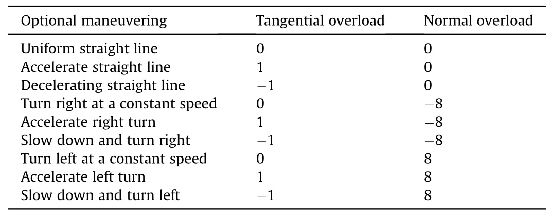
Table 1 Airplane action space.

2.2. Air combat situation assessment

2.2.1.Air combat situation description

The air combat situation is used to describe the relative position,speed and angle of the enemy and our aircraft.The state vector describing the air combat situation at time t in this paper isS(t)=[q(t) φ（t）,d(t) vr（t）,vb（t）,β(t)].The description of the air combat situation in the plane with height h is shown in the Fig.1:

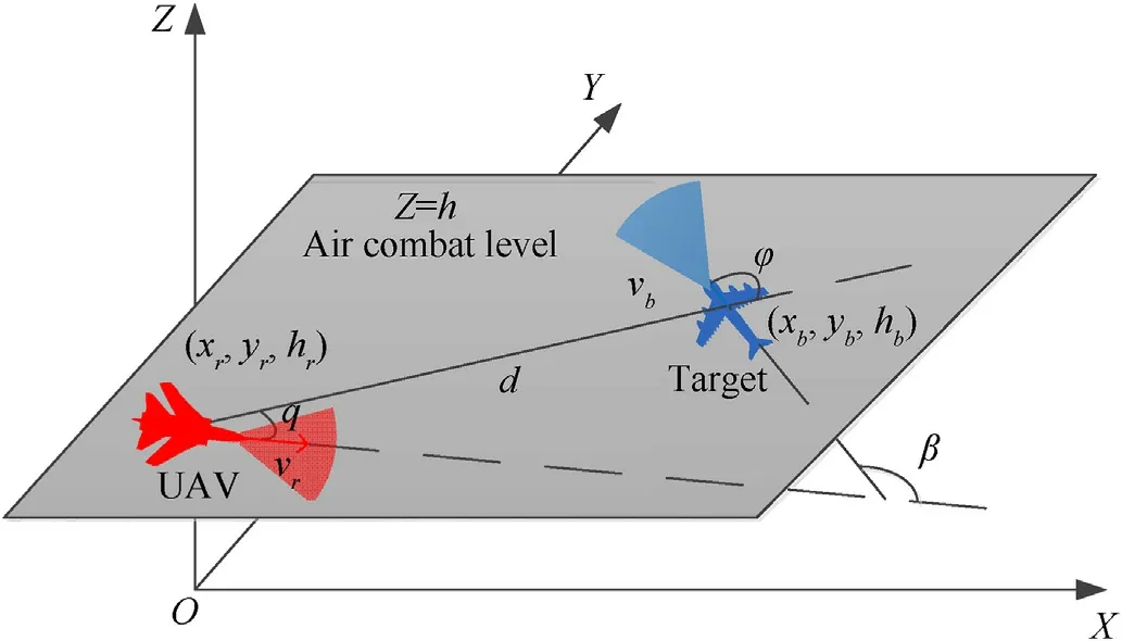
Fig.1.Air combat situation description.

The fan-shaped area shown in the figure is a simplified attack area of the UAV carrying the air-to-air missile,which mainly depends on the maximum range and off-axis angle of the missile.The positions of our UAV and enemy arePr=（xr，yr，hr）,Pb=（xb，yb，hb）;and vris the velocity vector of our UAV,vbis the velocity vector of enemy;d is the relative distance vector of both aircraft,pointing from our aircraft to enemy;qis the deviation angle of our aircraft,that is,the angle between our velocity vector andd;φ is the disengagement angle of enemy aircraft,the angle between the velocity vector of enemy andd;β is the angle between the velocity vectors of both aircraft.The six-dimensional state vector S=[q,φ,d,vrvb,β]can completely describe the situation of one-to-one air combat of UAVs in the horizontal plane.

2.2.2.Air combat situation assessment function

The air combat situation evaluation function is a standard for evaluating the current situation and is used to calculate the evaluation value (Eval) of the situation.Most of the existing research uses the evaluation value of the situation as the reward valueRin reinforcement learning to train the neural network.The air combat situation assessment function is composed of three sub-functions:relative distance advantage,speed advantage,and angle advantage.

(1) Angular Dominance Subfunctionf1

In air combat,it is believed that the closer you are to a tailchasing situation,the easier it is for the enemy to fall into our attack zone,and the greater our advantage will be.On the contrary,our UAV will be at a disadvantages.In this paper,the deviation angle and the departure angle are used to measure the angular dominance,and the angular dominance function is defined asf1

When the deviation angleqand the breakaway angle φ approach 0°,the angular advantage is the largest,and our aircraft is in a position of superiority;on the contrary,whenqand φ are close to 180°,the enemy aircraft has the advantage.

(2) Distance advantage subfunctionf2

The distance advantage is related to the maximum launch distance of air-to-air missiles.When we are behind the enemy's aircraft,we need the distance advantage function to guide the aircraft to approach the target.Use the distance between the two sides of the air combat to measure the distance advantage,and define the distance advantage function asf2

In the equation,dis the current distance between the two parties;σ is the standard deviation;dmaxmaximum launch distance of air-to-air missiles.

(3) Speed Advantage Subfunctionf3

When enemy aircraft is far away,our UAV needs to increase speed to approach the target;when the target enters our attack zone,our speed needs to be adjusted so that our aircraft can launch the missile stably.The optimal speed of our aircraft(v+)is related to the maximum launch distance of missile,UAV’s max-speed,and the target’s speed.Define v+as

In the equation,vbis the target speed,vmaxis the maximum flight speed of our aircraft,anddmaxis the maximum distance of the missile.Based on v+,the speed advantage function is defined asf3

(4) Subfunction Weight Settings

In order to improve the speed of network training,it is necessary to set different weight ratios for the sub-functions in different situational scenarios: when the distance between the enemy and UAV is far,increase the weight of the angle function;when the distance is appropriate,increase the weight of the angle to make our side form a tail-chasing advantage;finally,increase the weight of the speed function to make our aircraft reach the optimal speed for firing weapons.The weights of the evaluation functions in this paper are set as follows：

(5) Reward and penalty factor settings

In Eq.(9),the range of situation assessment isFε (0,1),and the assessment value interval is small.Setting the thresholds m and n divides the air combat situation into three parts: disadvantage (0,m),balance of power(m,n),and advantage(n,1).The range of the balance of power is large,so that the UAV can explore the environment as much as possible in the early stage of training;during the training process,when our aircraft falls into the disadvantage of air combat,a penalty factor p is given to reduce the probability of repeated mistakes;and when an advantage is achieved,a reward q is given to reinforce the strategy adopted in this training.In summary,the evaluation value(Eval)of the air combat situation in this paper is calculated as follows：

According to this equation,when the situation evaluation valueEval>(n+q),it is considered that the enemy falls within the range of our attack area,and our UAV is in a dominant position;on the contrary,whenEval<(m-p),our UAV is locked by the enemy and falls within the range of enemy’s attack area;otherwise,the two sides are in a state of balance.

3.DQN based on LSTM networks

3.1. RNN and LSTM networks

Recurrent Neural Network (RNN) is a network with feedback,whose present output is not only related to the current input,but also to the output of the previous moment.The neurons in the hidden layer of RNN are interconnected with each other,and the output information of the previous moment is stored for calculating the output of the current moment.Generally,the FNN and the RNN network are used in combination,as shown in Fig.2.

Fig.2.Recurrent neural network structure.

Fig.2 shows a three-layer neural network structure.After the hidden layer RNN is expanded,it is shown as a green square.The inputx=（xt-1，xt，xt+1）contains the input of the three times before and after,ando=（ot-1，ot，ot+1）is the corresponding output,the three weights(v,w,u)are equal.The data processing process of the RNN network shown in Fig.2 is as follows,at timet:

In the equation,htis the memory of the neuron after time t,whilestrepresents the memory after screening,andotis the output of the neuron at time t.F(x)is the activation function,which is used to filter and filter the effective information in the memory,andG(x)is the normalized output function of the network.It can be deduced that

The current memory can be obtained by weighting and filtering the previous memory and the current input,and the current output is directly related to the memory.This reflects the memorability of the RNN network,which is more dominant when dealing with data with strong continuity.

LSTM is a variant of RNN network with better long-term memory.Its internal design of input gate,output gate and forget gate is used to decide which information to keep or discard.Its neuron structure is shown in Fig.3 below:

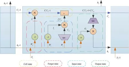
Fig.3.LSTM neuron structure.

In Fig.3,ct-1is the state information of the previous moment.After the information enters the neuron,it passes through the forget gateft,the input gateIt,and the output gateOtto obtain the current outputhtand the current cell statect,wherextis the input at timet,ht-1is the output of the neuron at the previous time,and the gate is a sigmoid function.

(1) Forgotten Gate: used to control the degree of information

retention inct-1,the calculation equation is as follows:

(2) Input Gate:add new memory based onct-1,CNis the newly generated memory,andItcontrols the degree of new memory addition

(3) Output Gate: After gettingct,this part produces the final outputht

The above is a single step of LSTM network processing data.Because of the existence of forget gate and output gate,LSTM network can selectively delete and retain information,which strengthens the ability of long-term memory.

3.2. RL in the field of motorized decision-making

Reinforcement learning is a process in which an agent continuously interacts with the environment to accumulate experience and correct mistakes.The general process of solving the Markov Decision Process (MDP) of reinforcement learning can be represented by a quintuple (S;A;P;R;γ).S is the state set;A is the optional action set;P（s，ai）is the probability of taking the actionaiin situation s;R is the action reward value;γ is the discount factor.Reinforcement learning is often combined with neural networks to make decisions.

The reinforcement learning process in the field of air combat maneuvering decision-making is shown in Fig.4: the initial situation and optional actions of both sides are set;our aircraft analyzes the situation and selects actions from the action library according to the output of the decision-making system;the enemy aircraft takes actions at the same time,and the two sides form a new round of Air combat situation;the situation assessment system calculates the evaluation value of the new situation,and deduces the return value of this decision;the generated return is used to revise the decision-making system.After continuous correction,the decisionmaking system can make a series of maneuvering decisions to guide our aircraft to occupy the air superiority,and then the training is completed (see Fig.6).

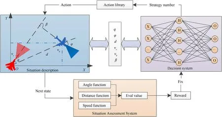
Fig.4.Reinforcement Learning in the field of motorized decision making.

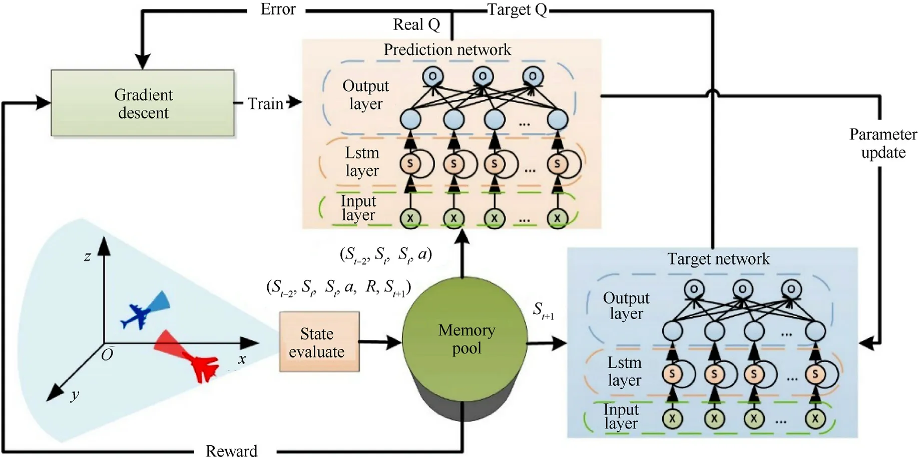
Fig.5.Improved DQN algorithm framework.

Fig.6.Air combat simulation process.

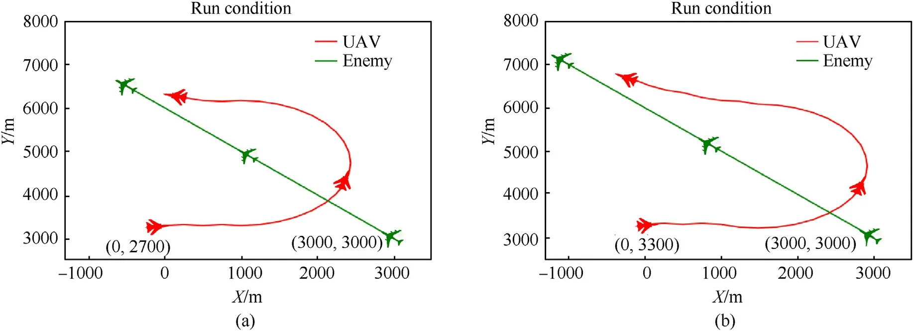
Fig.7.Engagement trajectory of both sides: (a) LSTM;(b) FNN.

Fig.8.Changes in the value of the posture evaluation: (a) LSTM;(b) FNN.

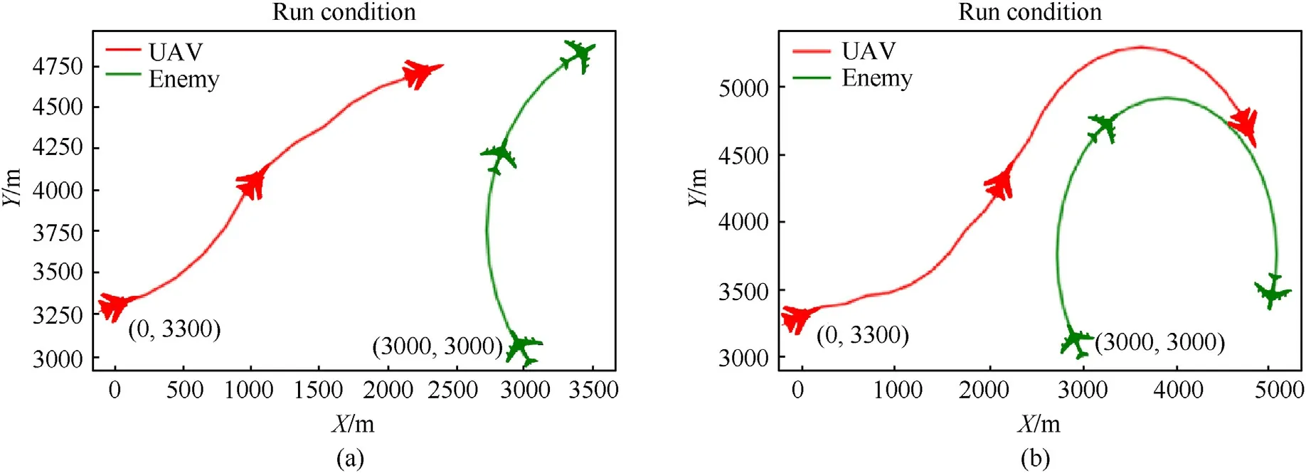
Fig.9.Engagement trajectory of both sides: (a) LSTM;(b) FNN.

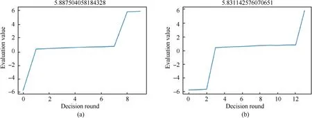
Fig.10.Changes in the value of the posture evaluation: (a) LSTM;(b) FNN.

3.3. Decision-making algorithms considering situational continuity

The algorithms in this paper makes an adaptive improvement based on DQN’ frame.The original DQN algorithm has three main characteristics:

(1) Approximate Value Functions with Neural Networks

DQN uses Temporal-Difference(TD)to calculate the currentV(s),and the algorithm in this paper uses a one-step lookahead value iteration

After training,the output of the prediction network will gradually approximate the true value function.For different input statess,the prediction network can outputQ（s，a）to simulate the real behavior value,solving the continuity problem of the state space.The neural network is trained by gradient descent,and its expression is

(2) Memory playback mechanism

Each time the agent explores the environment,it will obtain a data set(s,a,r,s΄),and the collected data sets are not independent and synchronized,and the existing correlation will lead to nonconvergence of training.The DQN algorithm reduces the correlation between data through the experience playback mechanism:the collected data is stored in the memory pool in sequence,and during training,a batch of data is extracted by random uniform sampling to train the network.

(3) Set up separate target networks

In order to enable LSTM to be trained under the DQN framework,adaptive improvement is required based on the above algorithm.Specifically,there are three changes as follows:

(1) Taking multiple situations as a single input to LSTM

LSTM can consider the continuity of the situation,but it has requirements on the format of the input data.In this paper,the situation of three consecutive moments（st-2，st-1，st）is used as the input of the network at timest,which reflects the Continuity of situation,also meet the requirements of the input format.

(2) Taking the difference in situation evaluation as the return value

In the field of air combat maneuver decision-making,the existing research mostly takes the evaluation value of the situation at the next momentEvalt+1as the return valueRof this decision.However,the pros and cons of a decision should not only be evaluated by the post-decision situationst+1,but also by the predecision situationst.Based on the establishment of the situation evaluation system,assuming that the evaluation value of the current situation isEvalt,and the evaluation value of the next situation after taking an action isEvalt+1,then the return valueRis set as

(3) Memory pool stores continuous situational information

Using the memory playback mechanism,DQN uses the information obtained by the agent as a sample to train the network.However,due to the requirements of the LSTM network for input data,each data in the memory pool needs to include the situation information at the previous moment.For LSTM network training,the data storage format in the memory pool should be（st-2，st-1，st，a，R，st+1）.

Based on the above three adaptive improvements,the framework for training the LSTM network in this paper is: take three consecutive air combat situations（st-2，st-1，st）as the input of the network,and the output is the strategy number;perform maneuvering actions according to the strategy number to obtain the next situationst+1;calculate the reward valueRaccording to the situation before and after;Put the collected data（st-2，st-1，st，a，R，st+1）into the memory pool;The data in the pool is sampled to train the prediction network and periodically update the target network parameters (see Fig.5).

4.Simulation

To verify the advantages of LSTM networks for processing continuous sequence data,the simulation in this paper is divided into four parts.The first part is conducted in a low adversarial scenario where the enemy trajectory is fixed,including two scenarios of uniform linear and uniform circling;the second part of the simulation is conducted in a scenario where the enemy performs a greedy strategy.In the first two parts,our UAV respectively uses LSTM and FNN to make decisions under the same conditions and verify the advantages of LSTM by comparison.In the third part of the simulation,the two sides of the air combat use different decision algorithms against each other,in which our side uses the algorithm of this paper and the enemy uses the algorithm of Ref.[27](referred to as TJ algorithm),and the advantages of the algorithm in this paper are verified through the match.The fourth part is selfconfrontation,the simulation is carried out under the condition that the initial situation,maneuverability,decision-making algorithm,and other factors of the both sides are completely consistent.

In addition,in order to make the simulation more in line with the scene of the UAV “dogfighting” in the actual air combat,the distance between the two UAVs should not be too far when setting the initial situation,and the speed should also be in a suitable range.

4.1. Simulation of the enemy flying along a fixed trajectory

The first part of the simulation is carried out in a simple scenario with low air combat confrontation to verify the possibility of the algorithm in this paper.In the simulation process,the enemy adopts two strategies of uniform linear and uniform circling respectively,and our aircraft adopts FNN and LSTM network for decision making respectively,and the simulation steps are specified as follows:

According to the above process,at the beginning of the air combat,this paper set the coordinates of the red aircraft(our side)Pr=（0，3300）,its speed vr=250 m/s,the heading angle θ=15°;the coordinates of the green aircraft(enemy)Pb=（3000，3000）,its speed vb=205 m/s,the heading angle θ=135°.The training will end after 50 rounds.The specific parameters of the simulation are as follows (see Table 2):

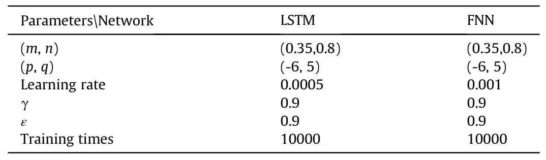
Table 2 Fixed trajectory simulation parameters.

The following picture shows the simulation results after the training is completed,in which the red line is the trajectory of our aircraft,the green line is the trajectory of the enemy aircraft,the left picture(a)is based on the LSTM,and the right picture(b)is based on the FNN network.

As shown in Figs.7-9 of the engagement trajectories,the two networks adopt roughly the same maneuvering strategies: at the beginning of the air combat,the two aircrafts are far apart,and our UAV is at a disadvantage state;then our aircraft continuously adjusts the heading angle and accelerates to approach the enemy;in the middle of air combat,our aircraft continues to accelerate and continuously corrects the course as the position of the enemy aircraft changes,making the situation from disadvantage to balance,and the evaluation value rises to (0,1);in the end of the air combat,our aircraft adjusted its speed after approaching the enemy,and the final evaluation valueEval>5.8,forming a tail-chasing advantage of stable tracking.The situation has experienced a disadvantage-balance-advantage change.

The changes in the evaluation value of each decision-making round of our side in the air combat are shown in Figs.8 and 10.Since LSTM can consider the continuity of the air combat situation,the number of decision-making rounds will be less in the same scene,and our aircraft can gain an advantage faster.This shows that the decision-making of LSTM is relatively efficient.

4.2. Simulation of the enemy executing greedy strategy

The simulation in the first part verifies the feasibility of LSTM network application in the field of air combat maneuvering decision,but the trajectories of enemy aircraft are determined in both scenarios,so the air combat is less adversarial.In order to analyze the performance of LSTM networks in more complex scenarios with certain adversarial nature,the second part of the simulation is conducted in this paper under the scenario where the enemy performs greedy strategy(see Fig.11).

Fig.11.Greedy policy decision process.

The greedy strategy will predict all possible next situationsst+1according to the current situationstand action space,then select the strategy corresponding to the situation with the highest score as the actual strategy after evaluating every possible situation.When executing the greedy strategy,the choice of maneuvering action needs to be determined according to the current situation,and the flight path of the target cannot be determined in advance,which increases the difficulty of training and is more practical.The decision-making process of the enemy's greedy strategy is as follows:

The setting of the initial situation of the air combat is the same as the previous scene:the coordinates of red aircraft(our side)Pr=（0，2700）,its speed vr=250 m/s,heading angle θ=15°;the coordinates of the green aircraft (enemy)Pb=（3000，3000）,and the initial velocity vb=205 m/s,its heading angle θ=135°;both sides have the same action space,but our UAV’s maneuverability is slightly higher.The training will end after 60 rounds,and the specific parameters of the simulation are as follows (see Table 3):

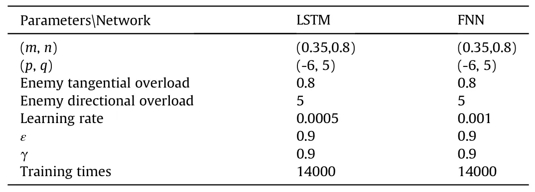
Table 3 Simulation parameters for Greedy Policy.

As the LSTM training progresses,the change of the engagement trajectory is shown in Fig.12 below.In the four trajectory’s diagrams,both fighters try to circle to the rear of the other side to form a dominant position,but our maneuverability is relatively dominant.After many staggered flights,our side takes a larger overload action to gain an advantage.

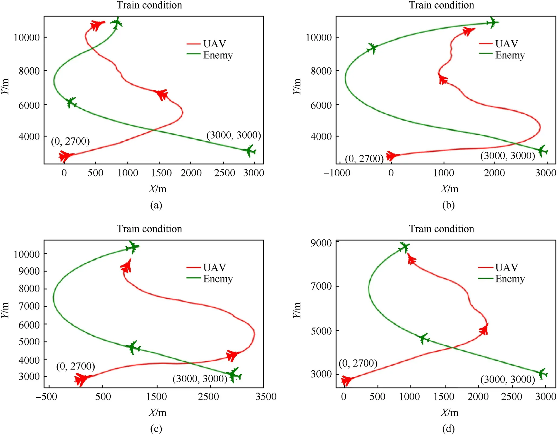
Fig.12.Trajectory changes during LSTM’s training: (a) Training times=5000;(b) Training times=8000;(c) Training times=10000;(d) Training times=12000.

The training times of the trajectory subgraphs (a)-(d) are gradually increasing.With the deepening of training,the air combat trajectory when our side wins are more concise,and the number of decision-making rounds gradually decreases.The following Fig.13 and Fig.14 are the simulation results after training,the left Fig.13(a) and Fig.14(a) is the LSTM network,the right Figs.13(b) and Fig.14(b) is the FNN network.

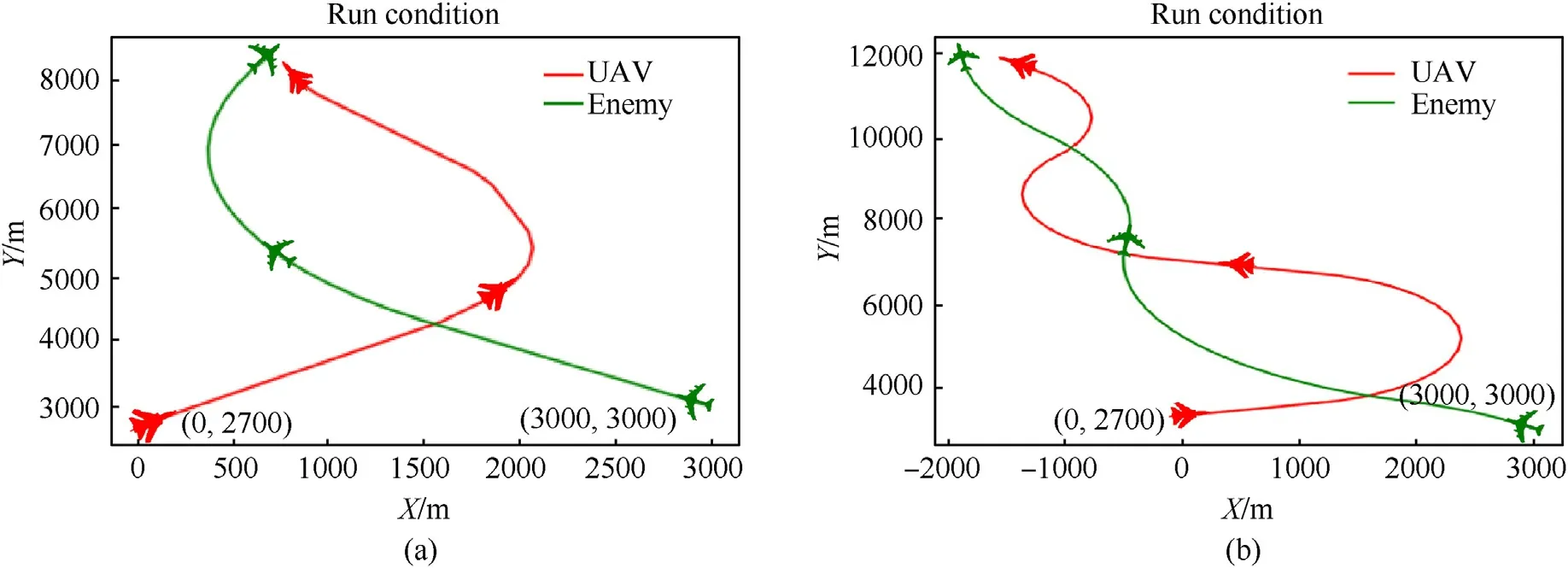
Fig.13.Combat trajectory comparison: (a) LSTM;(b) FNN.

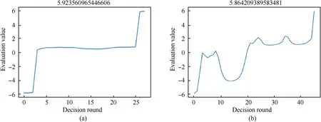
Fig.14.Comparison of changes in situation assessment: (a) LSTM;(b) FNN.

Figs.13 and 14 show that both networks can defeat the enemy after training,but the decision rounds of the LSTM network are relatively greatly reduced,and the average single-step decisionmaking efficiency is higher.

4.3. Simulation confrontation with TJ algorithm

The above simulation is a comparison of the same algorithm and different networks in the same scenario.The third part of the simulation is mainly about the confrontation between different algorithms.Ref.[27]proposes a maneuver decision-making method based on statistical principles (referred to as the TJ method).This method obtains possible air combat situations through maneuver testing,and makes maneuver decisions based on the expectation and standard deviation of the situation evaluation value.Our (red) UAV adopts the decision-making method based on situational continuity proposed in this paper,and conducts a one-to-one air combat simulation with the enemy (green)who uses the TJ method to make decisions.The enemy aircraft is set up with two different maneuvering performances,and the parameters of the two simulations are as follows (see Table 4):

Table 4 Simulation parameters for algorithmic confrontation.

The difference between the two simulations in the table above:the enemy maneuver performance is slightly lower than ours in simulation 1,the enemy and our UAV maneuver performance is identical in simulation 2,and the other parameters are identical in both simulations.In the simulation,the influence of the reward and punishment value is removed when evaluating our(red)air combat posture in the interval (0,1),while the evaluation of the enemy(green)air combat posture uses the evaluation function provided in Ref.[27].The following Fig.15 shows the changes in the evaluation values of the engagement trajectory and posture of both sides in the two simulations.

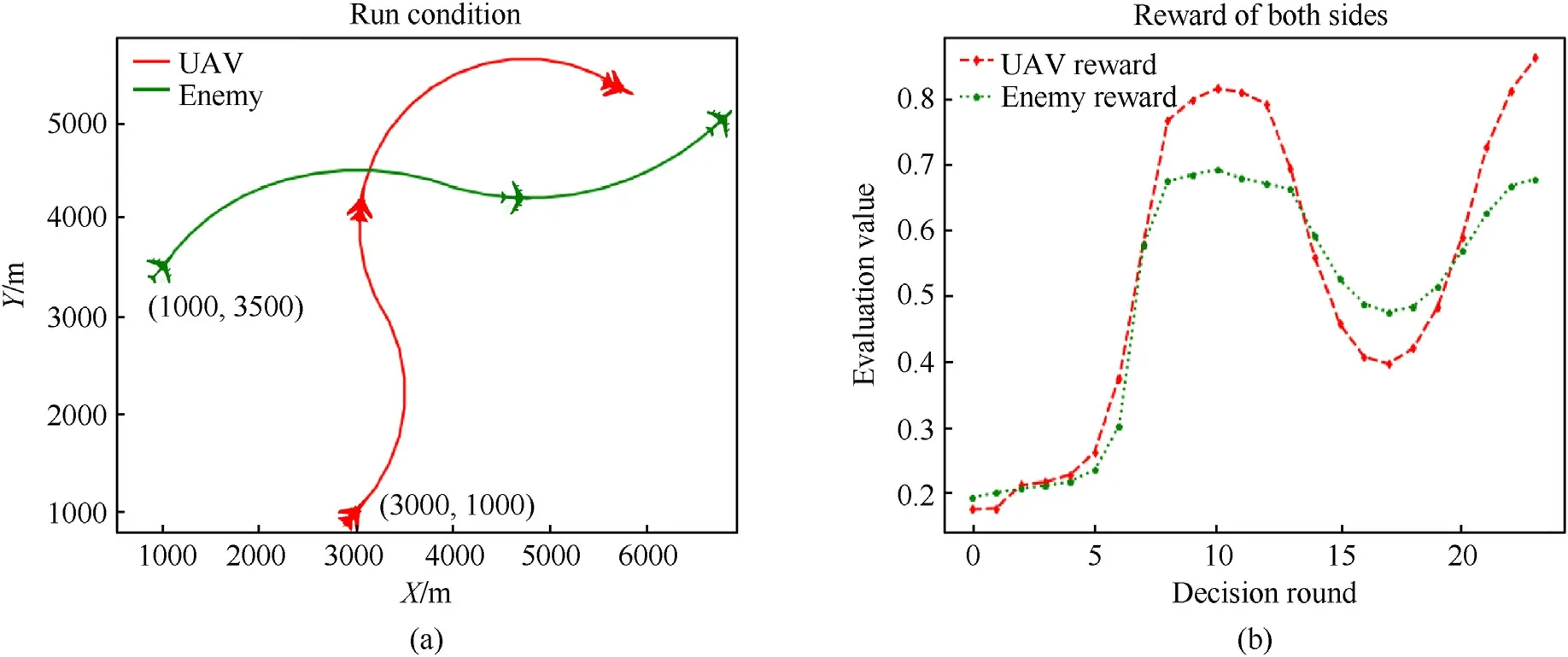
Fig.15.Simulation 1 Engagement Results:(a) Engagement trajectory;(b) Evaluation value.

Fig.16.Simulation 2 Engagement Results:(a) Engagement trajectory;(b) Evaluation value.

As shown in Figs.15 and 16,the initial situations of the two simulations are identical,and ultimately red UAV is the winner.However,due to the differences in enemy’s maneuverability,two engagement situations arise.At the beginning of the simulation,the two sides of the air combat were flying approximately in parallel,and the situational assessment values of both sides were at a low level.In the middle of the simulation,the two sides catch up with each other,and the evaluation value is very close.In the late stage of the simulation,when the enemy's maneuverability was lower than ours,as shown in simulation 1,our UAV defeated the enemy in 25 turns by a large overload maneuver.When the enemy's maneuverability is identical to ours,as shown in simulation 2,we are overwhelmed during the air combat,and it takes us about 35 rounds to defeat the enemy.

4.4. Self-confrontation simulation

The above three parts of the simulation are all comparisons or combats between the algorithm of this paper and other algorithms.The fourth part of the simulation designs a new scenario: the maneuver performance of the enemy and our UAV are identical,and both sides make decisions using the same algorithm proposed in this paper under the same initial posture.The simulation parameters are shown in the following table (see Table 5).

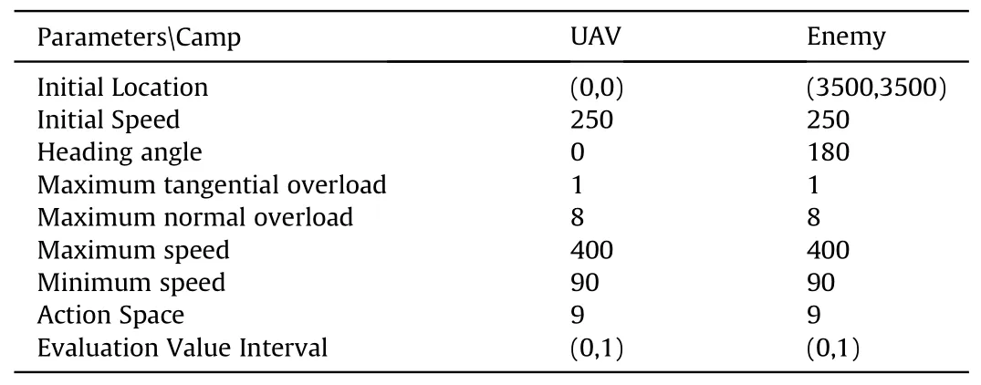
Table 5 Self-competition parameters.

The maximum number of rounds in this simulation is 60,and the simulation will stop when only one side UAV has the advantage,or when the maximum round is reached.The simulation results are shown in the following Fig.17,in which the left picture is the air combat trajectory,and the right picture is the change of the return value of each round of the two sides.

Fig.17.Self-competition result: (a) Engagement trajectory;(b) Evaluation value.

As shown in Fig.17 above,the changes in the air combat situation of the two sides are almost the same,and they can form launch conditions for each other at the same time,but neither can achieve an overwhelming advantage.The final simulation ends after reaching the maximum number of rounds.

4.5. Simulation analysis

(1) Comparison between LSTM and FNN

The first and second parts of the simulation were conducted in three scenarios based on LSTM networks and FNN networks respectively.Both networks were trained to obtain air combat victories,but with different numbers of decision rounds,as shown below(see Fig.18).

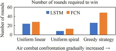
Fig.18.Comparison of the number of rounds required to win.

In three different scenarios,the decision-making rounds number of LSTM is less than that of FNN network,which shows decision-making based on LSTM network can achieve a dominant position through maneuvering in a shorter time.This shows that the LSTM network can consider the continuity between situations,its single-step decision-making is more efficient and forwardlooking,and it is more efficient in the global air combat range.In addition,as the air combat becomes more adversarial,the number of rounds needed to win the LSTM network decreases more dramatically,and the efficiency of decision-making becomes more apparent.

(2) Comparison between the algorithm of this paper and the TJ algorithm

The third part of the simulation is a confrontation between the two algorithms.Our UAV were able to win under the condition that the enemy had weak or normal maneuver performance,which also shows that LSTM's decision making is more effective and forwardlooking.The following Fig.19 shows the comparison of the decision time required by the two decision methods.The time data in Fig.19 are taken from 35 air combat rounds in simulation 2.The red line is the decision time of the algorithm proposed in this paper,and the green line is the decision time of the TJ algorithm proposed in Ref.[27].

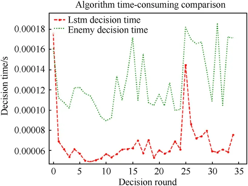
Fig.19.Decision time for both algorithms.

The above Fig.19 shows that the time required for each decision is floating for both algorithms.However,the algorithm used in this paper can output the policy value directly based on the situation,so its decision time is relatively shorter.The TJ algorithm requires a maneuver trial at each step before making decisions,so the decision takes a longer time.Theoretically,the more complex the UAV maneuver space is,the more rapidly the decision elapsed time of the latter grows.Therefore,compared with the TJ algorithm,the algorithm based on LSTM network decision making has higher air combat real-time performance.

5.Conclusions

Based on the simulation results of the above three parts,the following conclusions can be drawn:

(1) In the scenarios where the enemy flies along a fixed trajectory and executes a greedy strategy,the algorithm used in this paper can defeat the enemy.And compared with the FNN-based decision method,the decisions made by the algorithm in this paper are more efficient and forward-looking,and can achieve air combat dominance more quickly.

(2) With the improvement of scenario confrontation,the advantages of the algorithm based on situation continuity in terms of effectiveness and foresight will be more significant compared with the algorithm based on FNN.

(3) Under the condition that both sides have the same maneuver performance,the situation continuity-based decision method used in this paper is more effective and has higher real-time decision-making than the TJ algorithm in Ref.[27].

Declaration of competing interest

The authors declare that they have no known competing financial interests or personal relationships that could have appeared to influence the work reported in this paper.

Acknowledgements

This article is supported by the Natural Science Basic Research Program of Shaanxi (Program No.2022JQ-593).