pth-Moment Stabilization of Hybrid Stochastic Differential Equations by Discrete-Time Feedback Control

LU Yun(路 芸) , LU Jianqiu(陆见秋)

College of Science, Donghua University, Shanghai 201620, China

Abstract：The given unstable hybrid stochastic differential equation is stabilized in the sense of pth-moment exponential stability. We achieve the results by feedback controls based on the discrete-time state and mode observations. The upper bound on the duration between two consecutive observations is obtained as well. Finally, a numerical example is given to verify the validity of the theoretical conclusions.

Key words：Brownian motion; Markov chain; moment exponential stability; feedback control; exponential stability

0 Introduction

Hybrid stochastic differential equations (SDEs) with Markovian switching have been used to model many practical systems where they may experience abrupt changes in parameters and structures[1]. For example, financial and power systems affected by changes in structure or parameters can be characterized by SDEs[2].

A class of classical problems in hybrid stochastic systems is automatic control. In this field, many efforts have been devoted to investigating the stabilization of hybrid SDEs by regular feedback controls[3-5]. In general, scholars design a feedback control in the drift part to stabilize an unstable SDE based on continuous state observations as,

dx(t)=[f(x(t),r(t),t)+μ(x(t),r(t),t)]dt+
g(x(t),r(t),t)dB(t).

(1)

wherex(t) is the state of the system,r(t) is the mode of the system,fandgare referred to as the drift and the diffusion coefficients, andμ(x(t),r(t),t) is a feedback control based on the current state.

In order to reduce cost, Mao[6]proposed feedback controls based on discrete-time state observations to stabilize a given unstable hybrid SDE. This topic has drawn some attention since then[7-11]. He also obtained an upper bound on the duration between two consecutive observations.

Obviously, this is perfectly fine if the mode of the system is obvious (fully observable at no cost). For example, the stochastic differential equation is often used in a financial system where the mode represents the interest rate[12]. However, it could often be the case where the mode is not obvious and it costs to identify the current mode of the system. Therefore, it is necessary for us to design a controller whose states and modes are discrete to meet the practical requirements[13-16].

Under the condition of Global Lipschitz inf,g, andμ, Songetal.[17]studied the following controlled hybrid SDEs (a feedback control based on the discrete-time statesx(kτ) and modesr(kτ)

dx(t)=[f(x(t),r(t),t)+μ(x(δ(t)),
r(δ(t)),t)]dt+g(x(t),r(t),t)dB(t),

(2)

whereδ(t)=[t/τ]τ.It shows that if the SDE (1) is mean-square exponentially stable, then the SDE (2) is stable as long asτis sufficiently small. As we all know, many scholars have studied the mean square stability[18-22].

However, some practical problems need to study the higherpth-moment exponential stability. For example, in Refs. [23-24] the researchers studied thepth-moment stability of stochastic delay system and proved that the considered stochastic system had a unique global solution. Correspondingly, some problems only require a lower moment stability. Dongetal.[25]stated the necessity of studying the moment exponential stability ofp<2.Although lower moment stability can be derived from mean square exponential stability, the condition of mean square stability is too strong for almost sure exponential stability. Therefore, it is necessary to study the order of moments on a larger scale.

Considering that the observations may have a delay in practical problems, Hu[18]considered adding a feedback control with a time delay to stabilize the unstable stochastic system. In addition, the previous linear matrix inequalities (LMI) techniques required the feedback control to be linear or the system to be linear[26]. Hu[14]used a new approach to overcome this limitation. When the time delay is relatively small, the system ispth-moment exponentially stable (p>0).

Therefore, we try to study whether discrete-time feedback controls can also be applied to stabilize hybrid SDEs in the sense ofpth-moment exponential stability (p>0) in this paper. This article highlights two main contributions as follows.

1) Compared with employing a Lyapunov functional[26-27], the mathematical technique applied in this paper can investigate the exponential stability in the sense of a wider range of thepth moment (p>0).

2)Feedback controls are designed based on discrete-time state and mode observations in this paper. Compared with continuous time observations, discrete-time observations of state and mode cost less in practice. This makes the theory more likely to be applied in practice.

The writing route of this paper is as follows. Section 1 introduces the basic knowledge. Section 2 states the lemmas to prove thepth-moment exponential stability of controlled SDEs by discrete-time feedback controls. Section 3 illustrates the main result of this paper through the detailed proof process. Section 4 is the conjecture and how the theorem in this paper is implemented in the controller design. Section 5 introduces a numerical example to support our results. Section 6 makes a simple summary of this paper.

1 Preliminaries

Throughout this paper, we let (Ω,,{t}t≥0,P) be a complete probability space with a filtration{t}t≥0 satisfying the usual conditions (i.e., it is right continuous and0contains all P-null sets. LetB(t)=(B1(t),B2(t),…,Bm(t))Tbe anm-dimensional Brownian motion defined on the probability space. IfAis a vector or matrix, its transpose is denoted byAT.Ifx∈Rn, then |x|is the Euclidean norm. IfAis a matrix, we letbe its trace norm.A=max|Ax|:|x|=1 be the operator norm. If bothaandbare real numbers, thena∨b=max{a,b}anda∧b=min{a,b}.

Letr(t),t≥0 be a right continuous Markov chain on the same probability space and it takes values in a finite state spaceS={1, 2, …,N} with its generator Γ=(γij)N×Ngiven by

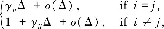
(3)

where Δ >0. Hereγij≥0 is the transition rate fromitojifi≠jwhile

(4)

Considering an unstable hybrid SDE

dx(t) =f(x(t),r(t),t) dt+
g(x(t),r(t),t)dB(t),t≥0,

(5)

where the statex(t)takes values inRnand the moder(t) is described by a Markov chain taking values in a finite spaceS={1,2,…,N},B(t)is a Brownian motion, andfis the drift coefficient,gis the diffusion coefficient. The coefficientsf:Rn×S×R+→Rnandg:Rn×S×R+→Rn×mare Borel measurable.

The purpose of this article is to design a Borel measurable control functionu:Rn×S×R+→Rnthat makes the followingn-dimensional hybrid SDE exponentially stable in thepth-moment

dx(t)=[f(x(t),r(t),t)+u(x(δ(t)),
r(δ(t)),t)]dt+g(x(t),r(t),t)dB(t),

(6)

whereδ(t)=[t/τ]τ.Hereτ>0 and [t/τ]is the integer part oft/τ.We only need to observe at discrete time0,τ,2τ,3τand so on. To make the hybrid SDE (6) have a unique solution, we impose the global Lipschitz condition.

Assumption1Assume that there are positive constantsL1,L2,L3such that

(7)

for all (x,y,i,t)∈Rn×Rn×S×R+.Moreover,

(8)

for all (i,t)∈S×R+.Condition (7) is for the stability purpose of this paper and condition (8) is for the existence and uniqueness of the solution[28]. We should point out that these conditions imply the following linear growth condition:

(9)

for all (x,i,t)∈Rn×S×R+.We claim that under Assumption 1, for any initial data

(10)

for allt≥0.

In fact, it is known that {r(δ(t,0,τ))}t≥0={r(kτ)}k≥0is a discrete-time Markov chain with a one-step transition probability matrix eτΓ.From the importance of the initial value, denote the solution byx(t;x0,r0, 0) and the Markov chain byr(t;r0, 0).Moreover, fort∈[0,τ], SDE (3) becomes a hybrid SDE

dx(t)=[f(x(t),r(t),t)+u(x0,r0, 0)]dt+
g(x(t),r(t),t)dB(t),

(11)

Repeating this procedure on time intervals [kτ,(k+1)τ] fork≥1, the arguments show that the process has the following property at the discrete timeskτ,k≥0

(x(t;x0,r0, 0),r(t;x0,r0, 0)) =x(t;x(kτ),

r(kτ),kτ), +r(t;r(x(kτ)),r(kτ),kτ),

(12)

For allt≥kτ, wherex(kτ)=x(kτ;x0,r0, 0) andr(kτ)=r(kτ;x0,r0, 0).

Let us consider the controlled hybrid SDE (2). To avoid confusion, we usey(t)for the state to distinguish it from the solution of the SDE (1). Considering the auxiliary controlled hybrid SDE

dy(t)=[f(y(t),r(t),t)+u(y(t),r(t),t)]dt+
g(y(t),r(t),t)dB(t),

(13)

ont≥0, write initial data

It is known that under Assumption 1, the SDE (13) has a unique solutiony(t) ont≥0.Meanwhile, it has the property thatE|y(t)|p<∞for allt≥0.

If we denote the solution byy(t)=y(t;y0,r0,0) , we put forward the following assumption about the solutiony(t).

Assumption2Assume that there is a pair of positive constantsMand γ such that the solution of the continuous-time controlled SDE (13) satisfies

(14)

Under this Assumption, the aim is to prove that the same control function also makes thepth-moment exponentially stable for the controlled system, provided thatτis sufficiently small.

2 Lemmas

To prove our main theorem, let’s first list some lemmas. It is important to emphasize that the following discussion is based onp>0.

Lemma 1 Under Assumption 1, for anyt≥0,

(15)

and

(16)

Specifically,

(17)

and

(18)

where

Ci(p) =

(19)

(20)

From Assumptions 1 and 2, we know

(21)

The second term on the right-hand side increases witht, so we get

The desired assertion holds under the well-known Gronwall inequality

Therefore,

Hence,

Taking the expectation on both sides gets the desired assertion formula (15).

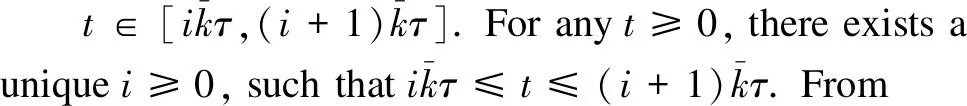
Then we can proceed to deduce formula (16) from Eq.(2) again. Note that ∀t≥0, there exists a unique positive integervfort∈[vτ, (v+1)τ).Thenδ(t)=vτholds for ∀t∈[vτ, (v+1)τ).Let’s consider the case ofp≥2,

Firstly, using the inequality(a+b)p≤2p-1(ap+bp),the above equation becomes the following inequality

And then using the theorem 7.1 in Ref. [4],

Then

Finally, repeating the similar steps whenp∈(0,2), we get

Lemma2[29]For anyt≥0,v>0, andi∈S,

(22)

where

(23)

Lemma 3 Let Assumption 1 hold. Fort≥0, writingy(t;y0,r0, 0)=y0,the following inequality holds,

(24)

where

(25)

(26)

dX(t)=[f(x(t),r(t),t) +μ(x(δ(t)),r(δ(t)),t)-f(y(t),r(t),t)-μ(y(t),r(t),t)]dt+

[g(x(t),r(t),t)-g(y(t),r(t),t)]dB(t).

(27)

Meanwhile, let

F(t)=f(x(t),r(t),t)+μ(x(δ(t)),r(δ(t)),t)-f(y(t),r(t),t)-μ(y(t),r(t),t).

(28)

(29)

where

(30)

M1(t)is a martingale withM1(0) = 0, soEM1(t)=0.Under Assumption 1, we begin to discuss the case ofp≥2.

(31)

where

u(x(s),r(s),s)]+[u(x(s),r(s),s)-u(y(s),r(s),s)]|ds≤J3(t)+

(32)

By Hölder inequality, we have

and from Lemma 1 and assertion (15)

So

Concretely,

(33)

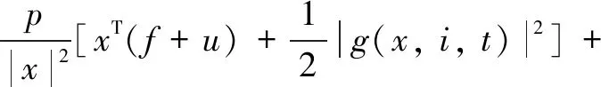
Letp0=0∨(p-1),∀kτ≤s≤(k+1)τby the well-known Fubini theorem, we definetk=kτfork=0,1,2…,

By Assumption 1 and conditional expectation∀tk≤s≤t∧tk+1,

(34)

From Lemma 2, we get

(35)

and we integrate it with

(36)

By Lemma 1, the inequality becomes

After the above deduction, we finally get

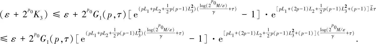
But there is still a part that needs to use the above Lemma 1, then bringK3into it

(37)

An application of the well-known Gronwall inequality yields

(38)

So whenp≥2,

Whenp=2,

Combining knowledge of conditional expectation, there must be

Therefore, the proof is complete.

3 Main Results

Under all the Assumptions and Lemmas, we can present our main theorem in this section.

Theorem1Let Assumptions 1 and 2 hold. Then there exists a positive numberτ*, such that the stochastic controlled hybrid system SDE (2) is exponentially stable in thepth-moment. That means ifτ≤τ*, then there is a pair of positive constantsCandλ, such that the solution of the controlled hybrid SDE (2) satisfies

(39)

It is important that we find out how to determineτ*.

Proposition1p0=0∨(p-1) has been defined in Lemma 3. We can choose a constantε∈(0, 1) andτ* is the unique solution of the equation.

(40)

whereγandMhave been given in Assumption 2. Obviously, whenτ=0,the left-hand-side term of Eq. (40) is 0. Meanwhile, it’s an increasing continuous function ofτint≥0.So Eq. (40) has a uique solution. In fact, we have no way to represent this number concretely. But with the help of the computer, we can find its value numerically. Note thatτ*followsε.If we can pick out a largerτ* with the value ofε, it would make a lot of sense in practice.

Then let’s begin to state the proof of Theorem 1.

ProofFork=0,1,2…,then we writekτ=tkandxkτ=xk,r(kτ)=rk.By the assertion formula (9), we know

x(t)=x(t;xk,rk,tk)∀t≥tk.

(41)

This implies

(42)

Furthermore, by the elementary inequality, (a+b)p≤2p0(ap+bp),a,b>0, we can deduce that

From Lemma 3,

so we get

(43)

(44)

so we have

Let the right part of the upper form beN(p,τ).

Through the assertion (40), we know

ε+N(p,τ)<1.

Therefore, ∃λ>0,

It then follows from formula (43)

Therefore,

(45)

holds. Then by Lemma 1 and assertion (45), whenp≥2

(46)

(47)

4 Enforcement

In this chapter, we consider how to enforce our theory. The given unstable hybrid SDE (5) needs a feedback controlu(x(t),r(t),t) in the drift. That can make the hybrid SDE (1) exponentially stable in thepth-moment. The form ofpth-moment stability has been shown in Assumption 2. There are plenty of documents that discuss how to determine the controller. In this paper, the controller is based on Ref. [3] and some conjectures are presented to enable Theorem 1 to be implemented.

Assumption3Letp>0.Assume that there are real numbersqi,i∈S, such that

(48)

for all(x,i,t)∈(Rn-0)×S×R+,while

H(p):=diag(q1,q2, …,qN)-Γ.

(49)

This a nonsingular M-matrix. Here’s an explanation of the M-matrix:H(p)=(hij)N×N,hij<0,i≠j,H-1>0.

Theorem2Under the conditions of Assumption 1 and Theorem 1, then Assumption 2 holds with

(50)

Consequently, Theorem 1 holds under Assumptions 1 and 3.

ProofWe observe that allqiare positive. Meanwhile,Ais a nonsingular M-matrix[24]. From the assertion (50), we know that

(51)

First, combining what we know from the theorem 5.8 in Ref. [24], we know that to make the SDE (1) stable, designing a Lyapunov function is necessary. Now we determine the initial value representation for Eq. (13). Lety(t0)=y0∈Rn, andr(t0)=r0∈S.Obviously, ify0=0, the equation holds, so we consider the case whenp>2 andr0∈Sarbitrarily and writey(t;x0,r0)=x(t).

within

Then,LV(x,i,t) is defined by

From Assumption 3, we get

However, by assertion Eq. (51), it’s easy to obtain

LV(x,i,t)≤0,EV≤V(x0,r0, 0).

(52)

Finally, substituting this into formula (52) yields

So

We now consider the general case: the controlled SDE (14) with the initial data

5 Examples

Example 1 Consider a two-dimensional hybrid SDEs

dx(t)=f(x(t),r(t))dt+g(x(t),r(t))dB(t),

(53)

whereB(t) is a scalar Brownian motion;r(t) is a Markov chain on the state spaceS={1,2}with the generator

Letx(t)=(x1(t),x2(t))T, then the coefficients of the HSDE are

The coefficients of the SDE are

By simulation (Fig.1), we can observe that the given SDE is unstable.

Fig.1 Simulation of the paths of r(t), x1(t) and x2(t) for the hybrid SDE using the Euler-Maruyama method with step size 0.001 and initial values: (a) r(0)=1; (b) x1(0)=-0.19; (c)x2(0)=1.4×1023

In order to prove that our theory can be applied to the stabilization of hybrid SDEs, we consider a uniform form of feedback control at first in this example. To make the later calculations easier, we design a linear control tox1.The form of linear control is as follows:

where all (x,i)∈(R2×S);e1ande2are both positive numbers to be chosen. It is not difficult to find that because of the coefficient characteristicf(x,i),g(x,i) of the equation, only the first statex1can be observed, the linear control of the two statesx1andx2is invalid.

From Assumption 1, we get

L1=0.2,L2=0.267 8,L3=0.2.

Therefore, we have

for(x,i)∈{R2-{0}}×S, where

After putting specific values into this expression, we get

The goal is to find the right valuese1ande2to stabilize the given SDE. Therefore, it is not difficult to find thatp<1 is an ideal case.

Now we consider the case whenp=0.98.Meanwhile, in order to make the calculation easier, we let 0.1-e1+0.02(p-1)=-0.1+0.005(p-1).Soe1=0.199 7.In the same way,e2=0.100 3.Consequently,

It is then easy to see thatq1=0.721 2 andq2=0.240 4.The nonsingular M-matrix defined by assertion (49) has the following form

It turns out that Assumption 3 is right whenp=0.98.It’s available nowβ1=5.591 9 andc2=5.732 5.Therefore, we getM=1.040 8 andγ=0.178 8 by Eq.(50).

By using Theorem 1 and Theorem 3, the solution of the uniform controlled SDEs

dy(t)=[f(y(t),r(t),t)+μ(y(t),r(t),t)]dt+
g(y(t),r(t),t)dB(t)

ispth-moment exponentially stable.

N(0.98,τ)=2p0K3(0.98,τ)=1-ε=0.2,

which has a unique positive rootτ*=7.340 8×10-8. By Theorem 1, the discrete feedback-controlled system

dy(t)=[f(x(t),r(t),t)+μ(x(δ(t)),
r(δ(t)),t)]dt+g(x(t),r(t),t)dB(t)

with the control functionμ(x,i,t) beingpth-moment exponentially stable as long asτ<7.340 8×10-8.Once again, the computer simulation (Fig.2) supports this theoretical result clearly.

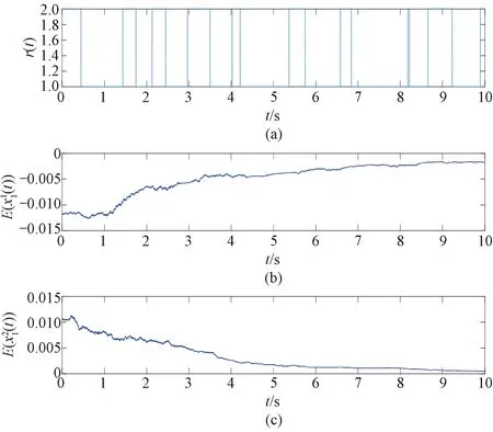
Fig.2 Simulation of the paths of r(t), x1(t), and x2(t) for the hybrid SDE using the Euler-Maruyama method with step size 0.001 and initial values: (a) r(0)=1; (b) x1(0)=-0.012; (c) x2(0)=0.010 5

6 Conclusions

In this paper, we prove that hybrid SDEs can be stabilized by feedback controls based on discrete-time state and mode observations in the sense ofpth-moment exponential stability (p>0).In addition, we obtain the upper bound for the duration between two consecutive observations.